New Excel Functions in Excel 2021
Every time when Microsoft excel launches a new version new excel functions are also been added there. Excel 2021 also has new functions like FILTER, SORT, SORT BY, UNIQUE, SEQUENCE. These all excel functions help us reducing our processing time. Let us see in brief what these functions are and how they work. Let us go through these New Excel Functions in Excel 2021.
FILTER function in excel
Excel FILTER function allows us to filter a range of data from a dataset based on some criteria. It is one of the New Excel Functions in Excel 2021. Let us understand first the syntax of Filter formula excel.
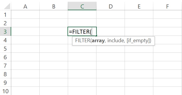
What we infer from the above image is that it requires 3 inputs out of which 2 are required. Let us understand each input one by one.
- array : array is the dataset from where we want to filter data.
- include : A Boolean array whose height or width is the same as the array
- [if_empty] : [Optional] The value to return if all values in the included array are empty (filter returns nothing).
Now understand this by an example. In this example, we have a dataset of sales done by sales agents. Data is bifurcated by Zone and quarter-wise. Out of this, we wanted to filter data for the North zone only.
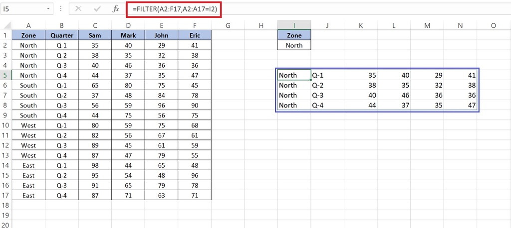
In the above example, we use excel filter function with array A2:F17 from where we will filter in excel. For the include option, we took array A2:A17 and matched it with our criteria which is available in I2. After closing the formula we get our filtered data. It starts from where we plug the excel filter function. It is to be noted here that it does not pick the header from the dataset.
Sort function in excel
Excel sort function helps in sorting the data from a dataset. It is the second among the new Excel Functions in Excel 2021. Though Microsoft Excel already has a sort option to sort excel data which sorts original dataset. Though this excel sort formula helps creates excel dynamic range. Let us first understand the syntax of how to use sort formula in excel.
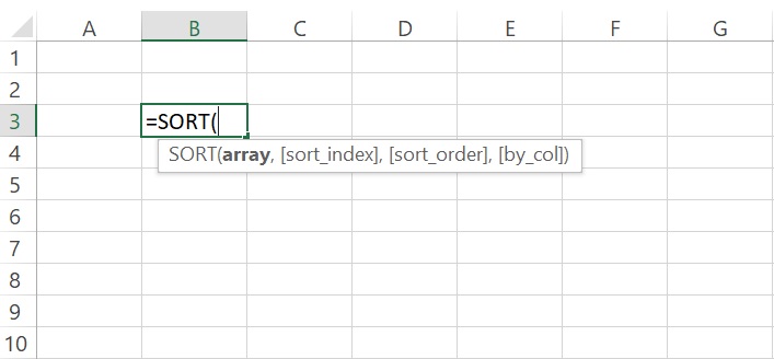
In the above image, we can see there are four inputs required for excel sort formula.
- array : The range or array which needs to sort.
- [sort_index] : Optional : A number indicating the row or column to sort by.
- [sort_order] : Optional : A number indicating the desired sort order. 1 for ascending order (default,if we missed to mention), -1 for descending order.
- [by_column] : Optional : A logical value indicating the desired sort direction. FALSE to sort by row (default), TRUE to sort by column.
Now let us go through an example to understand this.
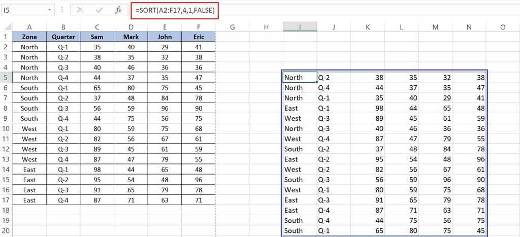
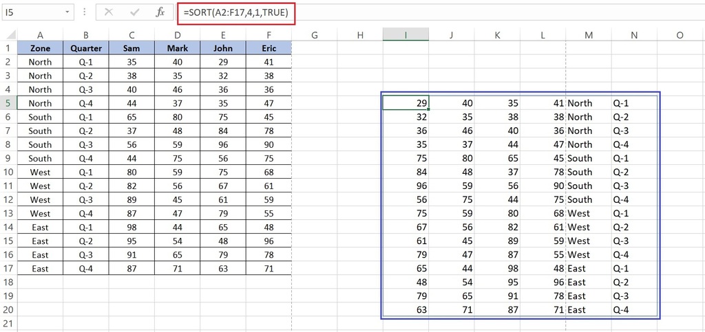
In the above image, we can see that we choose A2:A17 as our range which we wanted to sort. Now we wanted to sort the fourth column so we gave 4 as sort_index. In sort_order we put 1 as wanted to sort it ascending. Lastly, in [by_col] we put FLASE as wanted this sort by rows.
Now if you will see the fourth column the values are sorted in ascending order like 35,37,40,44 etc. Now let us check another example where we changed [by_col] value as TRUE while all other options remained the same.
SORTBY function in excel
Excel SORTBY formula is another newly added excel function. This is the third one in the new Excel Functions in Excel 2021. The SORTBY function sorts the contents of a range or array based on the values in a corresponding range or array. So you must be thinking what is the difference between sort and SORTBY function? Let me explain excel SORTBY function first then we will understand the differences between the both. Let’s first understand the syntax of SORTBY function.
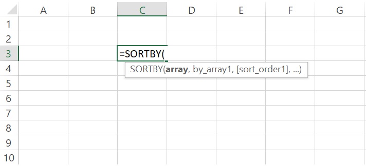
Can you guess how many inputs it required? Multiple! Yes. Let us discuss it in the below section.
- array : The array or range to sort
- by_array1 : The array or range to sort on
- [sort_order1] : optional: The order to use for sorting. 1 for ascending, -1 for descending. Default is ascending.
- [by_array2] : optional : The array or range to sort on
- [sort_order2] : optional: The order to use for sorting. 1 for ascending, -1 for descending. Default is ascending.
The above inputs are self-explanatory as we already explained earlier. In this function, just two inputs are required others are optional only. Also, we can observe that we can use multiple sort options in excel SORTBY function.
Now let us go through an example to understand it practically.
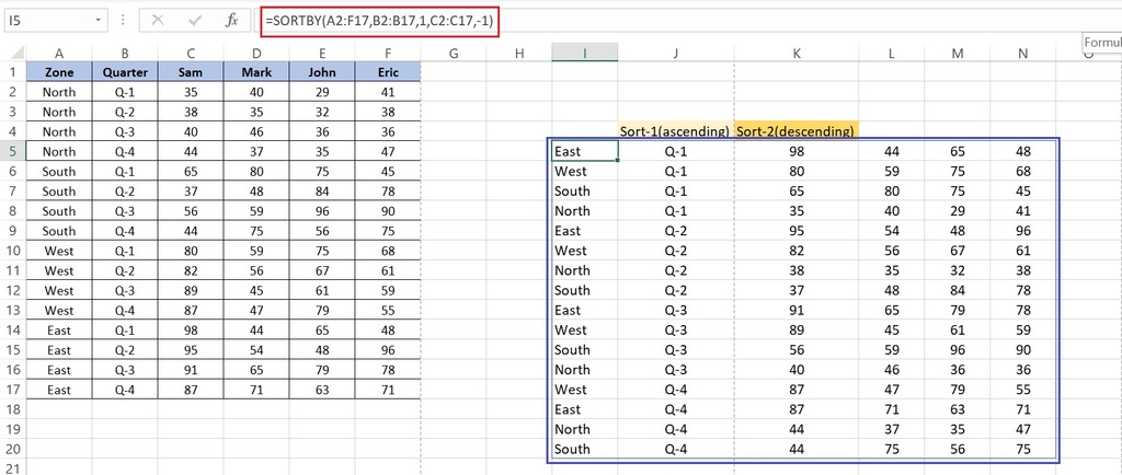
In the above example, we can see that the range or array to be sorted is taken as A2:A17. Next, we took reference for array which needs to sort B2:B17, and then put a value for [sort_order1] as ascending. And lastly, we took another array to sort as C2:C17 and use -1 for descending order in [sort_order2].
Difference between SORT function and SORTBY function.
- Excel SORT fucntion can sort by row or column but SORTBY function can be sorted by only rows.
- We can use only one option in SORT function though we can use multiple sort option in excel SORTBY option.
UNIQUE Function in excel:
The excel UNIQUE function returns a list of unique values in a list or range. This is the fourth of the New Excel Functions in Excel 2021. This is a very useful function as earlier we used to delete duplicate values in excel or used pivot table to make it unique and even used a very complicated formula to get a unique value list. Now by the use of the Excel unique formula, this task becomes very easy.
Let us first understand the syntax of excel UNIQUE function:
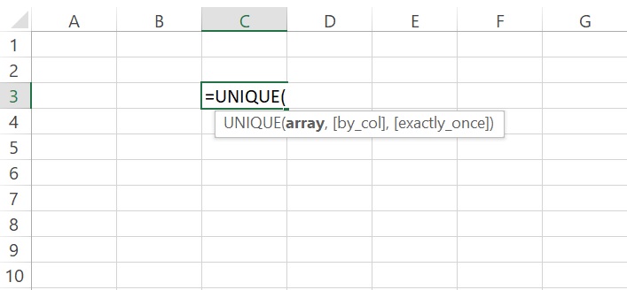
From the above image, we can infer UNIQUE function excel takes three inputs.
- array : The range or array from where we wanted to return unique rows or columns.
- [by_col] : optional : It is a logical value indicating how to compare.
- TRUE will compare columns against each other and return the unique columns.
- FALSE (or omitted) will compare rows against each other and return the unique rows.
- [exactly_once] : optional : This argument is a logical value that will return rows or columns that occur exactly once in the range or array. This is the database concept of uniqueness.
- TRUE will return all distinct rows or columns that occur exactly once from the range or array
- FALSE (or omitted) will return all distinct rows or columns from the range or array
Now we will go through an example so that we can get it correctly.
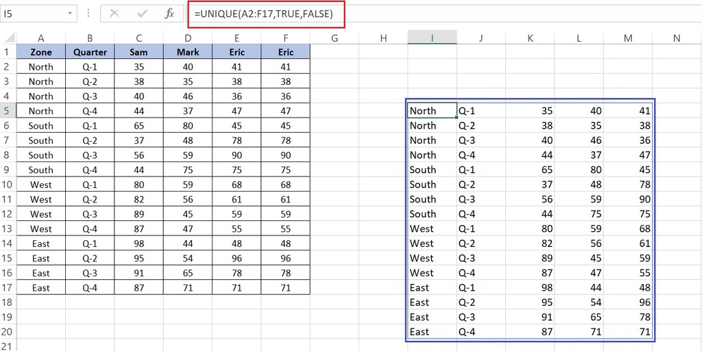
In the above example, we can see that we took A2:F17 as our range. In [by_col] we took value as TRUE as we wanted to match columns against each other. Finally, in [exactly_once] we took value as FALSE because we want one unique column out of the two same columns. Now if we see the blue highlighted area we found out of two duplicate columns now we have just one column left.
The fifth and the last in this blog is SEQUENCE function excel. This is the fifth of the new Excel Functions in Excel 2021 It allows us to generate a list of sequential numbers in an array, such as 1, 2, 3, 4 or 3,5,7,9 based on the inputs we used in excel SEQUENCE formula.
Let us understand the syntax for SEQUENCE function excel.
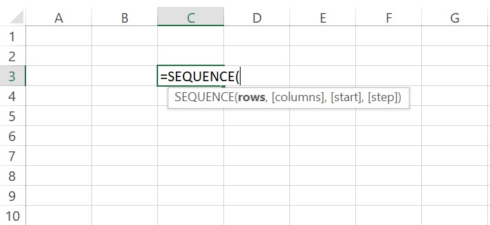
From the above syntax we can understand that excel UNIQUE formula need four input out of which 3 are optional.
- rows : The number of rows to return
- [columns] : optional : The number of columns to return
- [start] : optional : The first number in the sequence
- [step] : optional : The amount to increment each subsequent value in the array
Now let us get into an example to understand it properly.
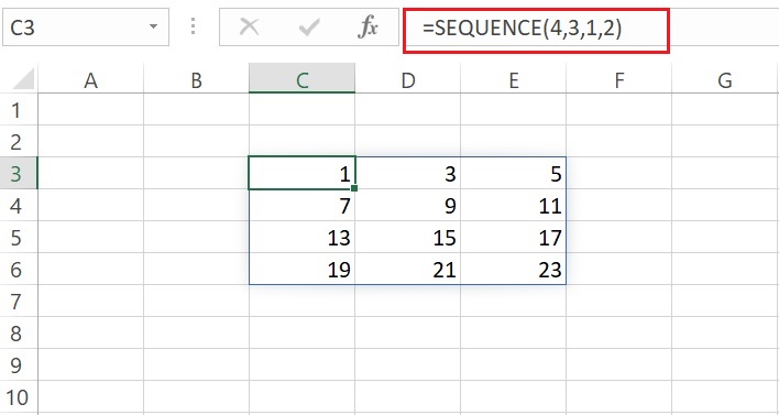
In the above example, we can see that we used four in rows value, which means we want four rows. While in columns we used three which means we wanted to create four columns. So it means we wanted to create a four by three table. Next in the start we put one which means we wanted to start with number one.
And finally, in the steps, we used two means we wanted our sequence with a gap of one. So finally we saw the result of our SEQUENCE formula is four rows by three columns which starts with one and sequentially increases by one value. The values move from left to right horizontally and then again start in the next rows.
That is all for now for New Excel Functions in Excel 2021. We will meet again with some new interesting functions or topics.
You can watch the below video as well where I had elaborately described this topic.
You can read more about New Excel Functions in Excel 2021 from the below articles which will definitely help you.

