Excel Slicer: How to use Excel slicer to filter data
What Slicer in excel
Slicers are floating buttons in excel by which we can filter data in an excel table or pivot table. In addition to this slicer reflects the current filter state means what options are selected currently. We can move slicers anywhere in the sheet and even can change their size and color.
How to create Slicer
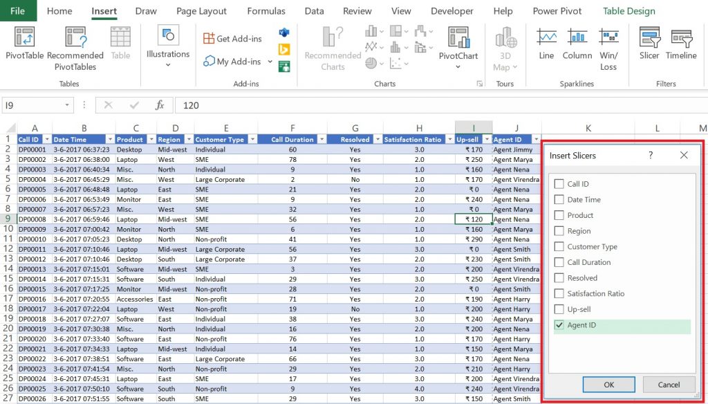
To create a slicer we need a pivot table or just an excel table. First, we need to go to the Insert tab in ribbon >> Filter section >> Slicer as shown in the below image.

Click on Slicer a new pop up option will come which will contain all column name of the table/pivot table. In this example have taken excel table to elaborate it.

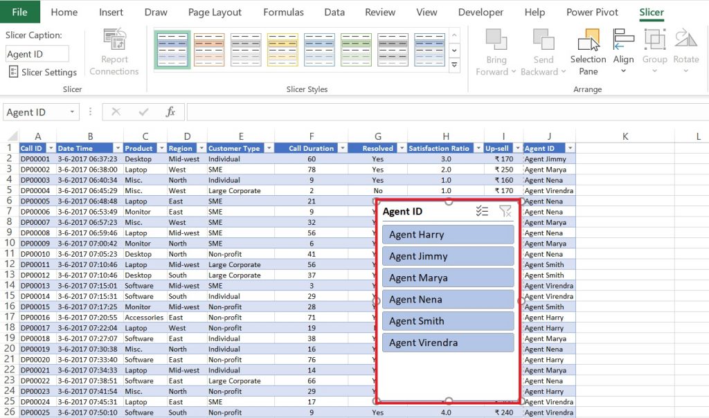
Choose an option(column name) from the pop up. In this example Agent ID.A new pop up will open and it will have all unique value of this column.

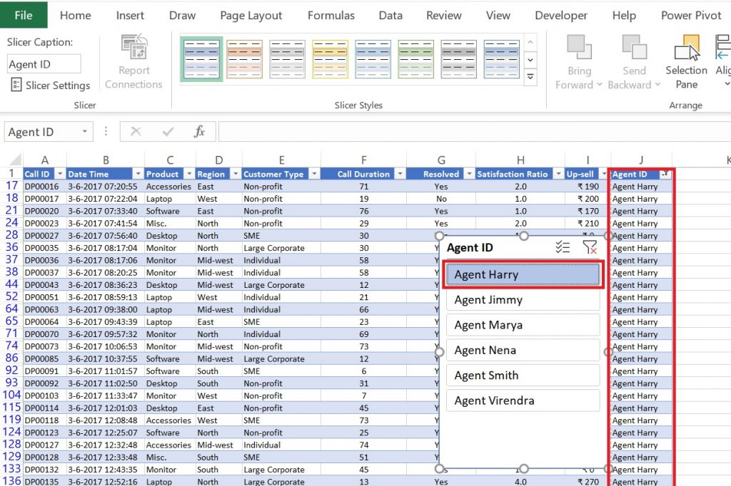
Now if we will select any option from this data will get filtered for this option only. I have selected Agent Harry in this option.

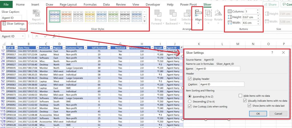
There are other options available by which we can control slicer. Like changing color & style, size, alignment of slicer. There is one more option available which is Slicer setting. It can help in changing name of slicer, display of header and hide items with no data.

There are more option to explore that I will leave on you to explore. That’s all for now will talk in next post.
https://www.excel-easy.com/examples/slicers.html
You can watch this video for better understanding on this.


Pingback: Excel Pivot Table: How to use it and its basic understanding - DataWitzz
Pingback: Table in Excel: How to create excel table step by step by 2 methods - Learning, we made it Easy