Excel Pivot Table: How to use it and its basic understanding

Excel Pivot Table

Pivot table is the most powerful tool of excel by which we can create a report or summarize our data in a very meaningful way. It is used usually with big datasets. In this article, we will be discussing the basics of Excel Pivot Table and step by step method to create Excel Pivot Table.

What is an Excel Pivot Table

We can think about Pivot Table as a report but it differs from the traditional reports which are static in nature. Pivot tables are interactive in nature and it is dynamic as well. We can group data into categories, filter data to include or to exclude some categories, can break date data into months or years and even we can create charts from it.

How to create Pivot Table in excel

To create a pivot table in excel we will select any cell on our dataset then we will go to the Insert tab then PIvot table and then in the drop-down click on Pivot table.

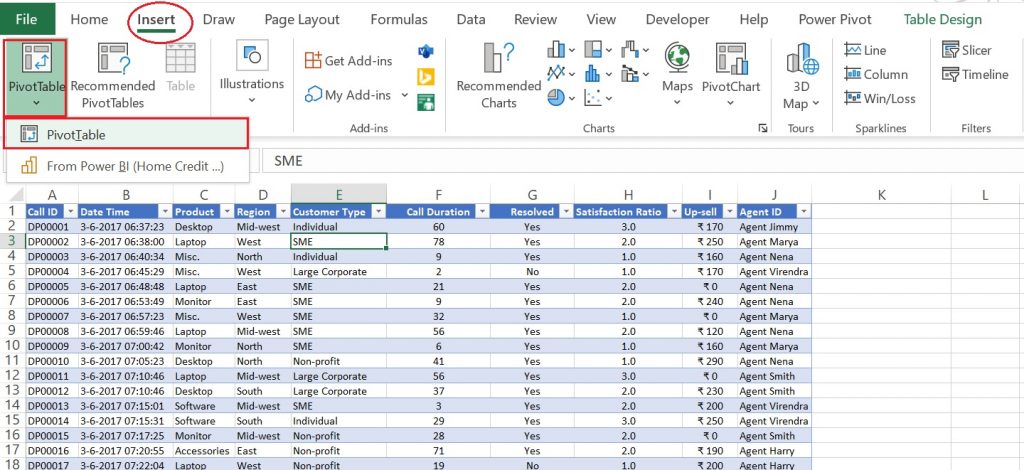
After choosing the above-mentioned options we will get a new pop-up box as shown in the below image.

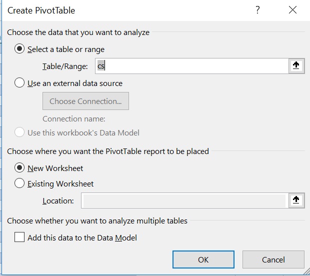
In the above image, we can see it asks to select a table or range. In our case, our data is in the table so we would give the name of the table. Then it asks for using an external data source which is not required in our case as we have our data already with us. Now it asks where you want to place the pivot table report. We can place it either in a new Worksheet or in the Existing Worksheet. For the existing worksheet, we need to provide the location. We will select a new worksheet. After selecting these options we will click OK.

Now after clicking OK we will be in a new sheet which will be looking like as below image.

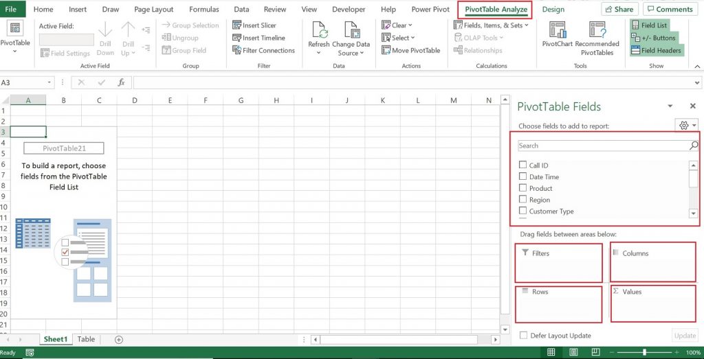
First option on the upper right side Choose fields to add to report has all columns of the data set and we can select any column name to show in our reports. In the lower right side we can see there are four boxes.Lets understand these options.

Filters: Filters are use filter our data. It will reflect at the upper left part and will contain different categorical values to select from. If we don’t select any value all dataset will reflect while if we choose a particular value it will reflect data for that value only. We can you Slicer as well to filter our data.

Columns: If we put a column in Columns box it will reflect all unique value horizontally from that column. It helps us to understand data for each unique value.

Rows: It also like Columns when we put a column in the Rows it will reflect unique values from that column.

Values: It shows values aginst the Columns and Rows value. There are multiple options by which we can Summaries value field by.

• Sum
• Count
• Average
• Max
• Min
• Product
• Count Numbers
• StdDev
• StdDevp
• Var
• Varp

Let us understand it by the below example.

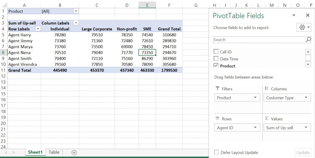
In the above example we have taken Product as a Filters,so we we will choose any product the value in the below table will get changed accordingly. In the below image when we choose Product as Accessories then all values in the table got changed.

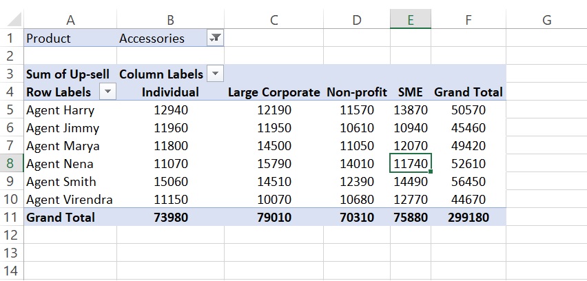
2nd thing we did is to choose Customer Type in columns. After choosing this we can see all unique values spread over as columns. It helps us to read value individually.

Now in the rows we put Agent ID so it reflects all agent ids.After that we put Up-sell in the Values box and choose Sum in the Summarize values as. Now it can see or read complete data. Some of the analysis we can infer here are below but not limited to those only.

• How many Up-sell was done by Agent Smith
• How many Up-sell was done by Agent Marya for SME Customer Type
• For Product Accessories how every operators Upsell the product

That is all for the introductory part of Pivot table in excel. Will write on Pivot tables in the next articles. Be connected.

For more on excel Pivot table we can read below articles.

• https://www.excel-easy.com/data-analysis/pivot-tables.html
• https://www.lumeer.io/pivot-table-complete-guide/