How to create excel table
Table in excel is a powerful feature that helps us in organizing our data by grouping data together. It is very quick to create a table in excel by just clicking a few keys or using a shortcut key and converting your flat data into a table with a lot of benefits.
The benefit of using excel table is as below but it is not limited to these only:
- Clean Formulas : When we are using excel table feature then it become very easier to read forumals even it is very complicated.
- Referencing a range : It is very easy to reference a range as every table has its own name.
- Auto expand : It is a feature of table in excel to auto update a column or row when we fill a cell.
- Quick Style : There are multipl formats are available for excel tables to make it more visual friendly.
- Filters and Subtotal : Automatically add filters and substotals to filter our data.
How To Make a Table in Excel
How To Make a Table in Excel
To make table in excel we will first select our dataset then will go to Insert then Table. Click Table option a new box will come that will ask the range of our dataset. After selecting the dataset range and if we have header of the dataset then check My table has headers. We can alternatively use ALT+T also which is a shortcut to create data table in excel.
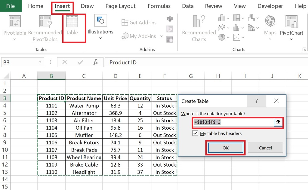
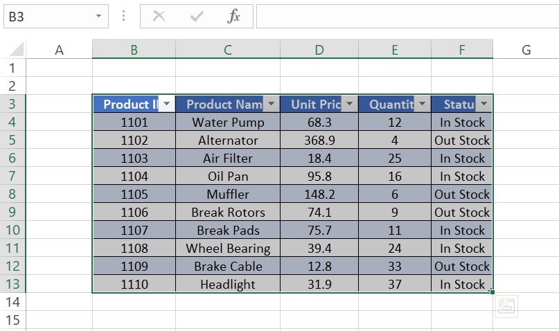
After clicking OK our dataset will get converted to excel table range as illustrated in the below image.
Working with tables in excel
As soon as excel table created, we also get a new table in the excel ribbon which Table Design. Excel table design is used to make multiple changes in table in excel and to create table styles in excel.
How to Use Table Styles in Excel
In the above image table is in blue and white table style. We can change it and choose any table style depending on our requirements.
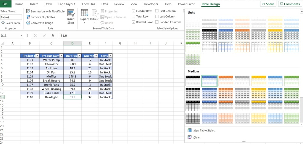
We can see different options here like Light, Medium, New Table Style, and even to clear the existing table design.
Table Style Options
This is a very useful option in excel table. By the use of these options we can make the following changes:
- Header Row: Used to show row of the table. If we uncheck it header row will delete.
- Total Row : It will activate excel Subtotal function at the bottom of the rows.
- Banded Rows: If we will uncheck banded rows option then strip of the table will get removed.
- First Column: It will highlight the first column of table.
- Last Column: It will highlight the last column of table.
- Banded columns : It will make abnded columns like we see for the rows.
- Filter Button: By unchecking this defualt filter will get removed.
How to Apply Table Names
When we create a table excel automatically picks table name. We can change this manually by write name by our choice as shown below. We need to go to Table Design then Properties. There we find Table Name.
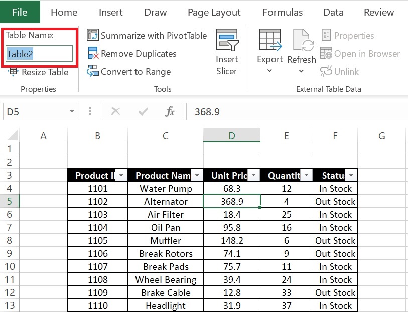
In the above image, we can change name of table as per our desire. It will help us to recall table name while referencing any table in any formula.
How to Use Excel Table Filters
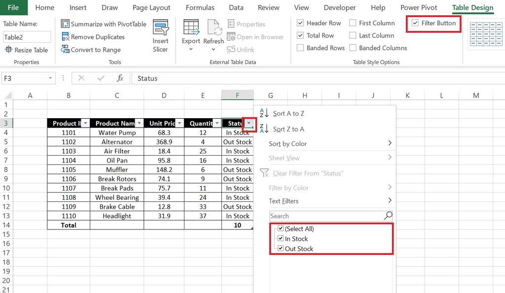
It is very easy as we mentioned earlier in table design that we have an option Filter Button in Table style option block. When we will check Filter Button option filter will reflect on the table headers. We can choose any option to filter our data.
How to Apply Subtotals in excel table
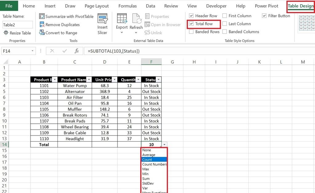
For activating Subtotal option we need to go to Table Design then go to table style options then check Total Row. We will get a new row at the bottom of the table. It will have different options for summarising out data like sum, average, Count, max etc. We can sum table column excel by using this option. It also has None option if we don’t want to use it for now.
How to use slicer in excel table
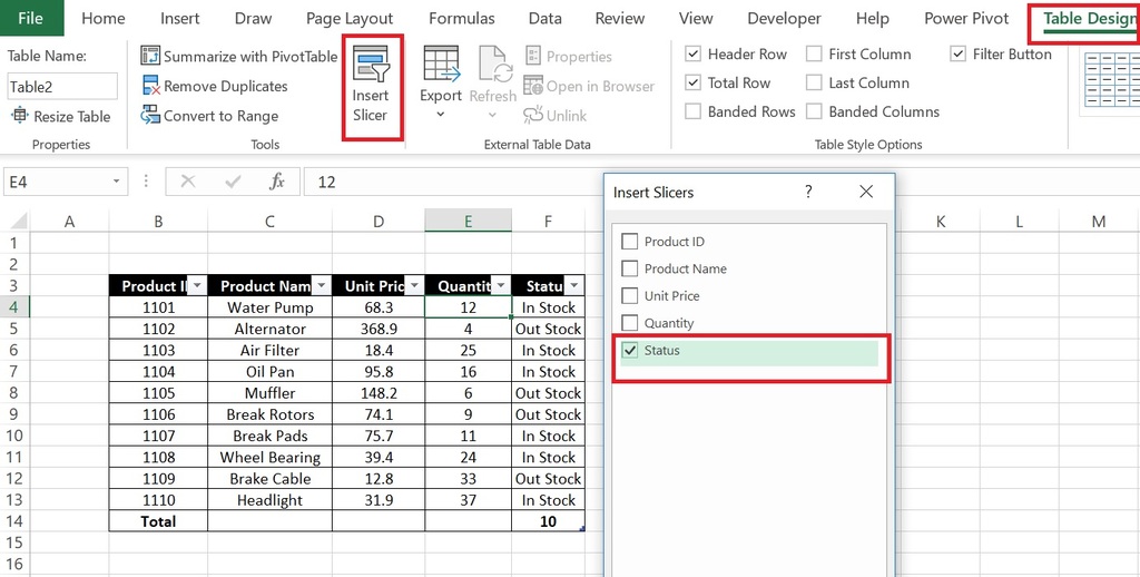
Like Pivot Table we can add slicers to filter the data in this table also. To use slicers in table we will first go to Table Design then click on Insert slicer. After clicking on Insert slicer we will get an option to choose a column name by which we wanted to filter our data. Choose a column option.
We will get a slicer of the column that we choose right now.
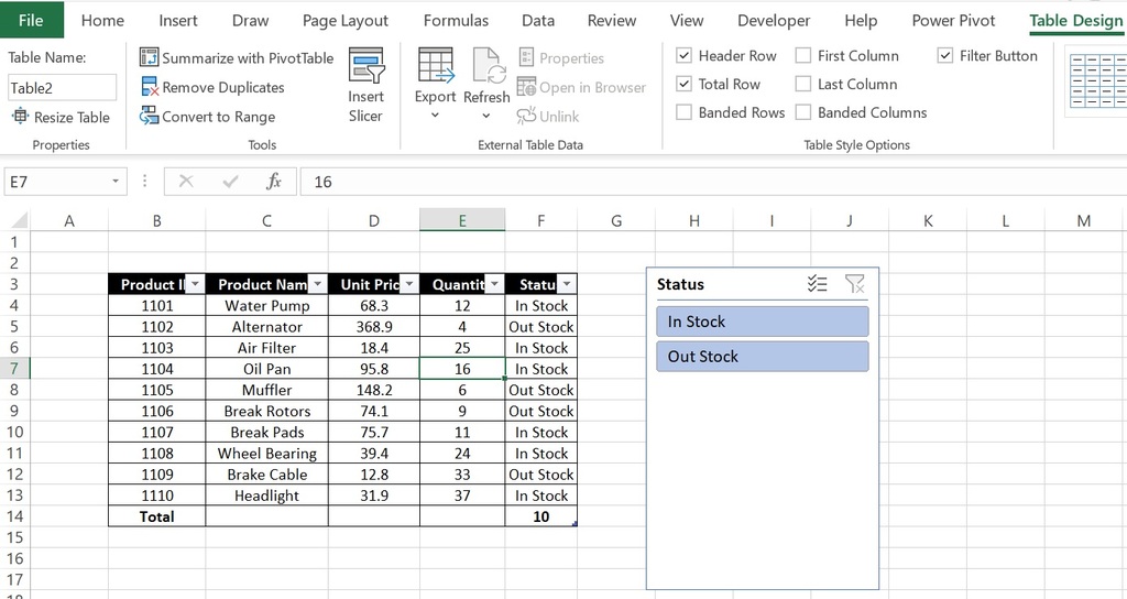
Now if we select any option here our data will get filtered for this option only.
That was all for how to make tables on excel. Will meet again with some new topics on excel.
You can read more on how to create a table excel by reading the below articles.
You can watch the below video also to get more clarity on it.
Excel table tutorial

