Index Function
Excel Index function is an excel function that comes under lookup and reference functions. Index function helps in getting a value from a reference or array. It also works like VLOOKUP but it edges higher as it lookup value from any side and even from a different array. It can be used along with other excel functions to get summary data.
There are two different ways by which we can use excel index function. Let us understand the syntax of index function
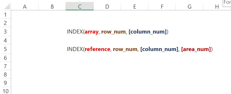
The first syntax array represents an array or range of data, row_num means the number of row from which data is supposed to pick if we miss this value or put 0 all rows will be selected and [column_num] is the column from where data needs to pick if we left blank or choose 0 value then it will default to all rows in the array provided.
The second syntax reference represents the array or range of data and it could be one or more. If we are selecting more than one range or area then we need to separate it by comma, row_num means the number of row from which data is supposed to pick if we miss this value or put 0 all rows will be selected and [column_num] is the column from where data needs to pick if we left blank or choose 0 value then it will default to all rows in the array provided. [area_num], if we select more than one range then we would use [area_num] and its number will be the sequence of ranges we had used in reference. If the value for [area_num] is omitted then the default value will be 1.
How to use the INDEX Function in Excel?
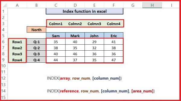
Let us understand it by two different examples but fore that let us understand the data.
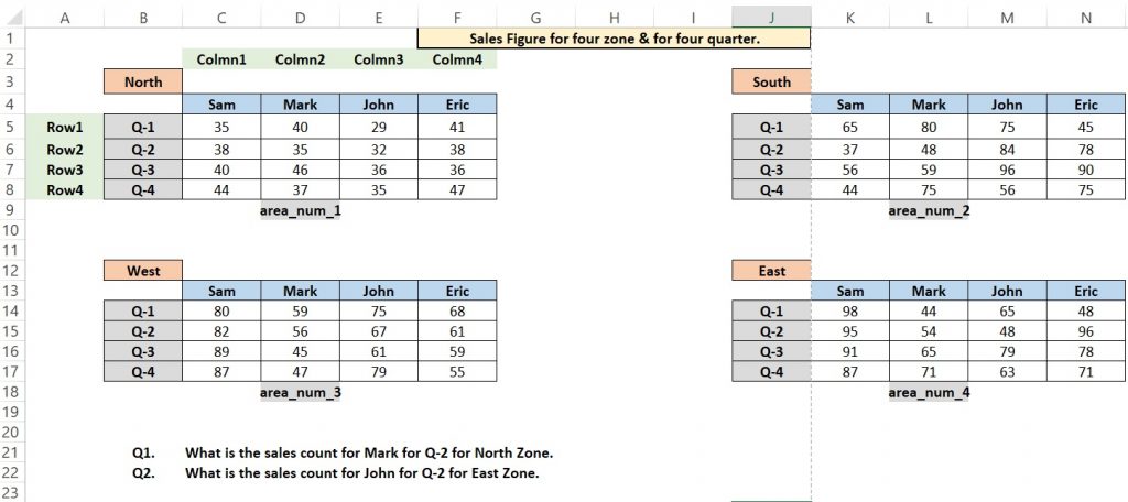
In the above image, we can see there are four sets of data that show quarterly data for sales agents for four zones. Also, we can see how the rows and columns are supposed to select. Now we will try to lookup value for Mark for Q-2 for North Zoone.
Using first index we will try to find value for this question, We also use excel MATCH function to find rows and columns.
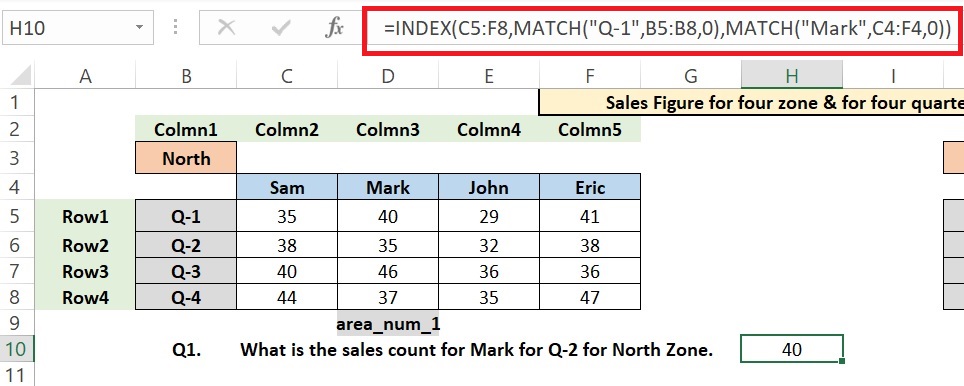
In the above image, we got a value of 40 for Mark for Q-1 for the North zone. Now let’s understand how we use the formula. We used the INDEX function and used C5:F8 (data portion of table) as an array, for rows and columns we used MATCH Function. If we wouldn’t want to use the MATCH function then we could use 1 as row_num and 2 as [column_num]. The index formula would be like =INDEX(C5:F8,1,2)
Now we would try to get an answer for the sales count for John for Q-2 for West Zone. To find this we would use the second index.
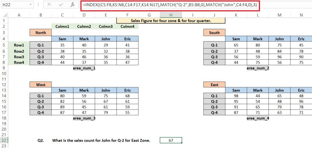
In the above image, we can see the value we get is 67. In this example, we use reference(multiple ranges) as can be seen in the red highlighted box. We first took range of North then south, then west and East. So as per the sequence West zone’s [area_num] will be 3. After that, we used the MATCH function to find out rows and column number. We can observe here the data in each array is in the same format.
That is all for this article. We will learn more about Excel INDEX and MATCH function’s uses in the coming blog.
You also can read more on Index from the below Articles.


Pingback: How to use MATCH function in Excel - Learning, we made it Easy