If you’ve ever needed to sum data based on a condition in Excel, SUMIF is the formula that gets the job done. Whether you’re an entry-level analyst or a seasoned finance professional, mastering SUMIF and its variations can save you hours every week and transform how you work with data.
In this comprehensive guide, you’ll discover 10 practical SUMIF examples — from the basic syntax to advanced tricks like wildcards, date ranges, dynamic references, and OR logic — all explained with real-world datasets. We’ve also included a free downloadable Excel practice file so you can follow along and try every formula yourself.
📥 Download the Excel Practice File
All 10 SUMIF examples with sample data are included in the practice workbook.
Let’s start from the beginning and build your SUMIF skills step by step.
What Is the SUMIF Function in Excel?
The SUMIF function in Excel is used to sum values in a range that meet a specific condition or criterion. It belongs to Excel’s family of conditional functions — alongside COUNTIF, AVERAGEIF, and SUMIFS — and is one of the most widely used functions in data analysis, accounting, and reporting.
SUMIF Syntax
=SUMIF(range, criteria, [sum_range])
Here’s what each argument means:
- range — The cells you want to evaluate against the criteria (e.g., a column of region names or product categories).
- criteria — The condition that must be met. This can be a number, text, cell reference, or expression (e.g.,
"North",">500","*Apple*"). - [sum_range] — Optional. The cells to actually add up. If omitted, Excel sums the range itself.
When to Use SUMIF
SUMIF is ideal whenever you need to answer questions like: “How much revenue came from the North region?”, “What’s the total sales for products over $500?”, or “What did we spend on marketing this quarter?” It’s the go-to tool for conditional summation in Excel without needing pivot tables or complex array formulas.
Example 1: Basic SUMIF — Sum by Category
The most fundamental use of SUMIF is summing values that match an exact text string. Let’s say you have a sales table with regions and want to total sales for just the “North” region.
Sample Data
| Region | Sales Rep | Sales Amount ($) |
|---|---|---|
| North | Alice | 4,500 |
| South | Bob | 3,200 |
| East | Carol | 5,800 |
| North | Eve | 6,100 |
| South | Frank | 4,400 |
Formula
=SUMIF(A2:A13, "North", C2:C13)
This tells Excel: “Look at column A. Wherever you find ‘North’, add up the corresponding value in column C.”
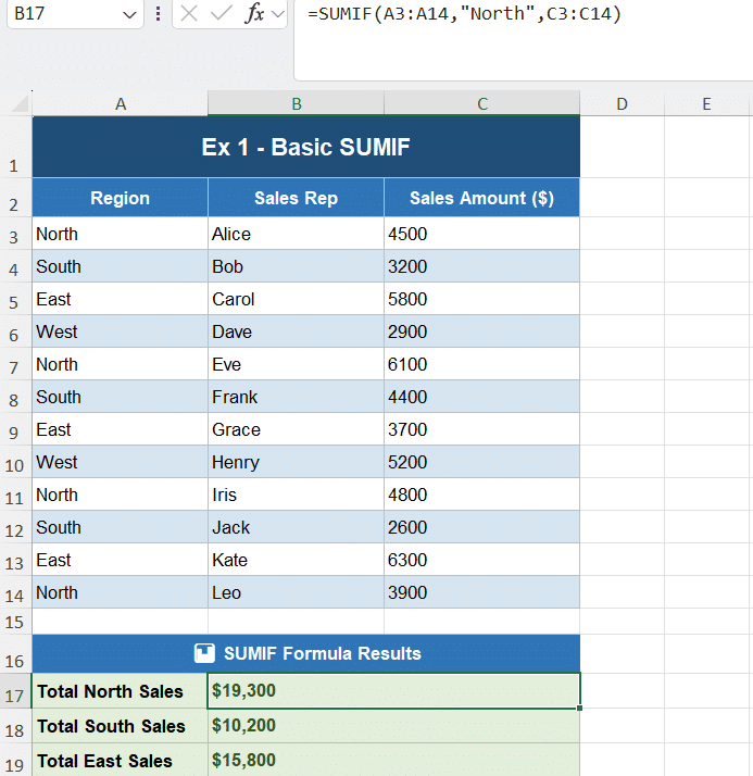
Result: $19,300 (sum of all North region sales)
Key Takeaway
For exact text matching, put the criteria in double quotes. SUMIF is not case-sensitive, so “North”, “north”, and “NORTH” all return the same result.
Example 2: SUMIF with Wildcard Characters (* and ?)
Wildcards make SUMIF incredibly powerful for partial text matching. Excel supports two wildcard characters:
- * (asterisk) — Matches any sequence of characters
- ? (question mark) — Matches exactly one character
Use Case: Sum All “Apple” Products
=SUMIF(A2:A11, "Apple*", C2:C11)
 2")
This formula will sum revenue for every product whose name starts with “Apple” — including Apple iPhone 15, Apple MacBook Air, Apple Watch Ultra, and Apple AirPods Pro.
More Wildcard Patterns
| Criteria | Matches |
|---|---|
"Apple*" | Starts with “Apple” |
"*Pro" | Ends with “Pro” |
"*Pro*" | Contains “Pro” anywhere |
"A???e" | 5 chars starting with A, ending with e |
Pro Tip: To search for a literal asterisk or question mark, use a tilde (~) before it: "~*"
Example 3: SUMIF with Comparison Operators (>, <, >=, <=)
You can use SUMIF with comparison operators to sum values based on numerical conditions. This is extremely useful in sales commission tracking, performance analysis, and financial reporting.
Use Case: Sum Commissions for High Performers (Units > 500)
=SUMIF(B2:B11, ">500", C2:C11)
This sums commission amounts only for employees who sold more than 500 units.
 3")
Comparison Operator Quick Reference
| Operator | Meaning | Example |
|---|---|---|
> | Greater than | ">500" |
< | Less than | "<100" |
>= | Greater than or equal | ">=500" |
<= | Less than or equal | "<=1000" |
<> | Not equal to | "<>0" |
Important: Always wrap comparison operators AND their values in double quotes: ">500" not >500.
Example 4: SUMIF with Date Ranges
Date-based SUMIF is one of the most powerful tools for financial analysis and reporting. The trick is combining operators with the DATE() function using the & (ampersand) concatenation operator.
Use Case: Sum Sales in the Second Half of 2024
=SUMIF(A2:A11, ">"&DATE(2024,6,30), C2:C11)
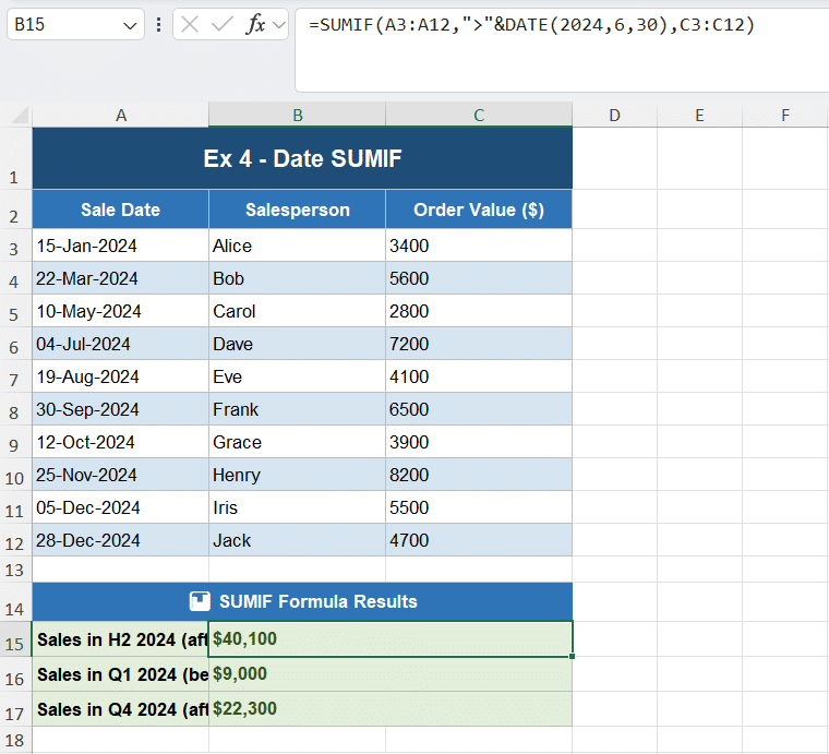
This sums all order values where the Sale Date is after June 30, 2024 — i.e., July through December 2024.
Why Use DATE() Instead of a Text Date?
Hardcoding dates as text (like "7/1/2024") can cause issues depending on regional date formats. Using DATE(year, month, day) ensures Excel always interprets the date correctly, regardless of locale settings.
More Date Formulas
=SUMIF(A2:A11, ">="&DATE(2024,1,1), C2:C11)    ' Sales from Jan 1, 2024 onwards
=SUMIF(A2:A11, "<"&DATE(2024,4,1), C2:C11)     ' Sales before Apr 1 (Q1 only)
=SUMIF(A2:A11, ">"&TODAY()-30, C2:C11)          ' Sales in last 30 days
Pro Tip: Use TODAY() for rolling date windows that automatically update every day.
Example 5: SUMIF for Blank and Non-Blank Cells
Data quality issues are common in real-world datasets. SUMIF can help you analyze incomplete data by targeting rows where a column is empty or has a value.
Sum Where a Cell Is Blank
=SUMIF(B2:B11, "", C2:C11)
Sum Where a Cell Is NOT Blank
=SUMIF(B2:B11, "<>", C2:C11)
 5")
Practical Applications
- Find total sales for orders with missing customer segment data
- Calculate revenue from transactions that have no assigned rep
- Identify and quantify data entry gaps in your records
Important Note: Cells with spaces (” “) are NOT treated as blank by SUMIF. Only truly empty cells qualify for the "" criteria.
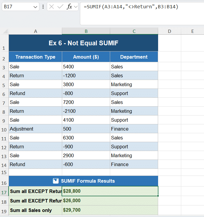
Example 6: SUMIF “Not Equal To” — Exclude Specific Values
The <> operator in SUMIF lets you sum everything except a specific value. This is perfect for excluding returns, refunds, cancellations, or any category you want to filter out.
Use Case: Total Revenue Excluding Returns
=SUMIF(A2:A13, "<>Return", B2:B13)
This adds up all transaction amounts except those categorized as “Return.”
Combining with a Cell Reference
=SUMIF(A2:A13, "<>"&D1, B2:B13)
Here, D1 contains the value to exclude. Change D1 and the formula dynamically updates — no need to edit the formula itself.
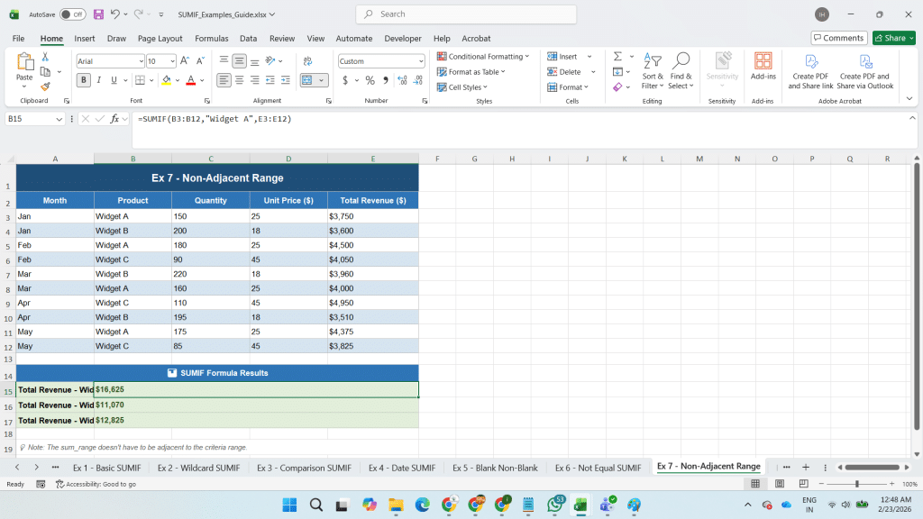
Example 7: SUMIF Across Non-Adjacent Columns
A common misconception is that the sum_range must be adjacent to the criteria range. In reality, SUMIF can reference any range in your spreadsheet — as long as the ranges are the same size.
Use Case: Sum Revenue by Product (Criteria in Column B, Revenue in Column E)
=SUMIF(B2:B11, "Widget A", E2:E11)
Here, column B contains product names, columns C and D contain quantity and unit price, and column E contains the calculated revenue. SUMIF comfortably bridges across the gap.
Rule to Remember
The criteria_range and sum_range must have the same number of rows and columns. Excel automatically aligns them from the top-left cell of each range.
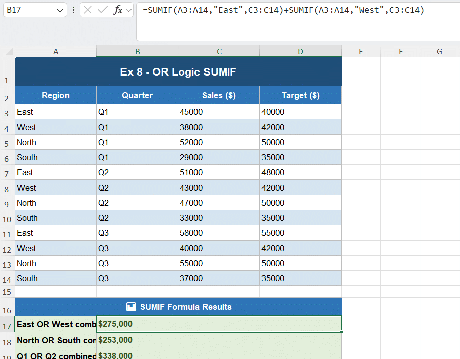
Example 8: Adding Multiple SUMIF Formulas for OR Logic
SUMIF natively handles one criterion at a time. For OR logic (sum if condition A or condition B), the simplest approach is to add two SUMIF formulas together.
Use Case: Combined Sales for East OR West Regions
=SUMIF(A2:A13, "East", C2:C13) + SUMIF(A2:A13, "West", C2:C13)
This gives you the total sales for both East and West without creating a helper column or pivot table.
Alternative: Using SUMPRODUCT for OR Logic
=SUMPRODUCT(((A2:A13="East")+(A2:A13="West")>0)*C2:C13)
SUMPRODUCT is more flexible for complex OR conditions across multiple columns, but for simple cases, adding two SUMIFs is cleaner and easier to read.
Example 9: Dynamic SUMIF Using Cell References as Criteria
One of the most analyst-friendly tricks is making SUMIF dynamic by referencing a cell for the criteria instead of hardcoding it. This turns your formula into a mini lookup dashboard.
Static vs. Dynamic Criteria
| Type | Formula | Limitation |
|---|---|---|
| Static | =SUMIF(C2:C11,"New York",D2:D11) | Must edit formula to change city |
| Dynamic | =SUMIF(C2:C11,G3,D2:D11) | Change G3, formula auto-updates |
Building a Simple Lookup Dashboard
Place your criteria values in a highlighted cell (like a dropdown using Data Validation), and point your SUMIF at that cell. As the user changes the dropdown, every SUMIF that references it instantly recalculates — no manual formula editing needed.
=SUMIF(C2:C11, G3, D2:D11) ' G3 = selected city from dropdown
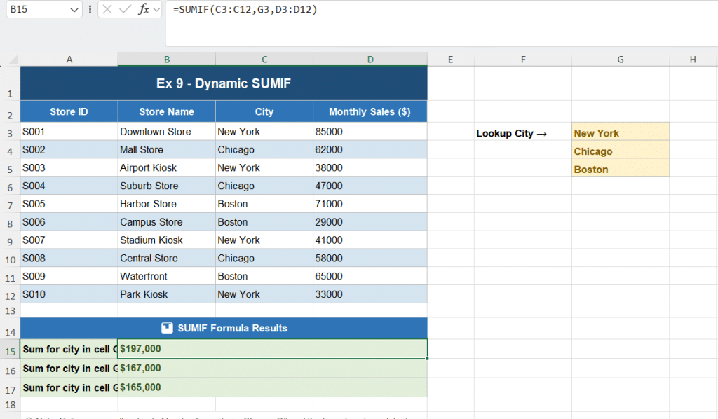
This pattern is the foundation of many professional Excel dashboards and management reports.
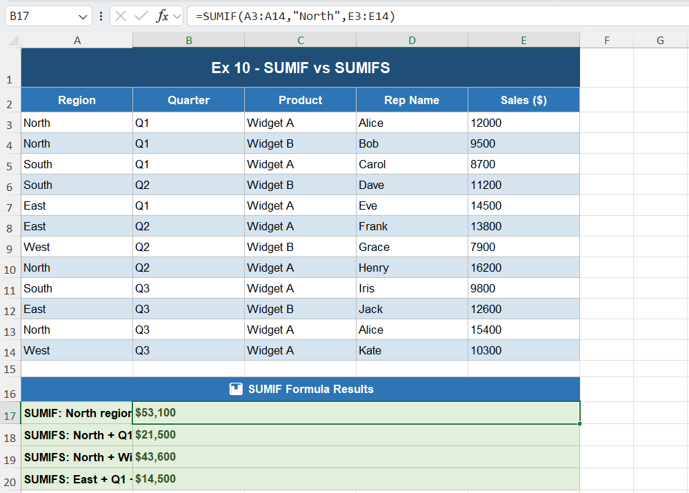
Example 10: SUMIF vs. SUMIFS — When You Need Multiple Criteria
While SUMIF handles one condition, SUMIFS is its more powerful sibling that supports multiple criteria simultaneously (AND logic). Every analyst should know when to switch from SUMIF to SUMIFS.
SUMIFS Syntax
=SUMIFS(sum_range, criteria_range1, criteria1, [criteria_range2, criteria2], ...)
Comparison Example
' SUMIF: North region (all quarters)
=SUMIF(A2:A13, "North", E2:E13)

' SUMIFS: North region AND Q1 only
=SUMIFS(E2:E13, A2:A13, "North", B2:B13, "Q1")

' SUMIFS: North AND Q1 AND Widget A
=SUMIFS(E2:E13, A2:A13, "North", B2:B13, "Q1", C2:C13, "Widget A")
Key Differences: SUMIF vs. SUMIFS
| Feature | SUMIF | SUMIFS |
|---|---|---|
| Number of criteria | 1 | Up to 127 |
| Logic type | Single condition | AND logic (all must match) |
| Argument order | range, criteria, sum_range | sum_range FIRST, then pairs |
| Availability | Excel 2003+ | Excel 2007+ |
| OR logic support | No (use + trick) | No (use SUMPRODUCT) |
Critical Note: In SUMIFS, the sum_range comes FIRST — unlike SUMIF where it comes last. This is a common source of errors when switching between the two functions.
🎯 SUMIF Excel Knowledge Quiz
Test your understanding of SUMIF formulas • 7 Questions
📋 Question Summary
Bonus: 5 SUMIF Pro Tips Every Analyst Should Know
1. Use Entire Column References for Scalability
=SUMIF(A:A, "North", C:C) ' Instead of A2:A100
Using full column references means you never have to update your formula when new rows are added. The slight performance trade-off is negligible for most datasets.
2. Combine SUMIF with INDIRECT for Sheet-Level Analysis
=SUMIF(INDIRECT(H1&"!A:A"), "North", INDIRECT(H1&"!C:C"))
Where H1 contains a sheet name. This lets you pull SUMIF results from different sheets dynamically.
3. Array SUMIF for Multiple Criteria Results at Once
=SUMIF(A2:A13, {"North","South","East","West"}, C2:C13)
This returns an array of four results — one for each region — useful when combined with SUM or in spill-enabled Excel 365.
4. Avoid Common SUMIF Errors
- #VALUE! — Usually caused by criteria_range and sum_range being different sizes
- Wrong results — Check for leading/trailing spaces in your data using TRIM()
- 0 when expecting a result — Verify the data type (numbers stored as text won’t match numeric criteria)
5. SUMIF Performance Tip
For large datasets (50,000+ rows), consider using helper columns or Power Query instead of multiple volatile SUMIF formulas, as they can slow down workbook recalculation.
Frequently Asked Questions About SUMIF in Excel
Q1: What is the difference between SUMIF and SUMIFS?
SUMIF evaluates a single condition (one criteria range and one criterion), while SUMIFS supports multiple conditions simultaneously using AND logic. SUMIFS also has a different argument order — the sum_range comes first in SUMIFS but last in SUMIF.
Q2: Can SUMIF handle OR logic (sum if A or B)?
Not directly. The most common workaround is to add two SUMIF formulas: =SUMIF(A:A,"East",C:C) + SUMIF(A:A,"West",C:C). For more complex OR conditions, use SUMPRODUCT.
Q3: Why is my SUMIF returning 0 when data exists?
The most common causes are: (1) numbers stored as text in your sum_range, (2) leading or trailing spaces in your criteria_range cells, (3) criteria case that doesn’t match (though SUMIF is generally case-insensitive), or (4) the criteria range and sum range being different sizes.
Q4: Is SUMIF case-sensitive?
No. SUMIF treats uppercase and lowercase letters as identical. “North”, “NORTH”, and “north” all match the same cells. If you need case-sensitive matching, use SUMPRODUCT with EXACT().
Q5: Can I use SUMIF with dates?
Yes. Use comparison operators combined with the DATE() function: =SUMIF(A:A,">"&DATE(2024,6,30),B:B). You can also use TODAY() for dynamic rolling periods.
Q6: How do I use SUMIF with wildcard characters?
Use * for any number of characters and ? for exactly one character. For example, "Apple*" matches any cell starting with “Apple”, and "*Pro*" matches any cell containing “Pro” anywhere. To match literal * or ?, prefix with tilde (~).
Q7: What is the maximum number of criteria in SUMIFS?
SUMIFS supports up to 127 criteria range/criteria pairs. In practice, if you need more than 5-6 conditions, consider using a different approach such as Power Query, helper columns, or a database.
Q8: Can SUMIF reference another sheet?
Yes. Use the syntax: =SUMIF(Sheet2!A:A, "North", Sheet2!C:C). Include the sheet name followed by an exclamation mark before the range.
Q9: Does SUMIF work with filtered/hidden rows?
No. SUMIF sums all matching rows regardless of whether they are hidden by a filter. If you need to sum only visible rows, use SUBTOTAL or AGGREGATE functions instead.
Q10: How do I make SUMIF ignore errors (#N/A, #DIV/0!) in the sum_range?
SUMIF automatically ignores error values in the sum_range — it simply skips them. However, errors in the criteria_range can cause issues. Wrap the criteria_range in IFERROR() if needed, or clean your data first.
Conclusion: Master SUMIF, Master Your Data
SUMIF is one of Excel’s most versatile and widely-used functions. From basic category summation to dynamic dashboards and date-based analysis, the ten examples in this guide cover the essential SUMIF patterns that every analyst encounters in the real world.
Here’s a quick recap of what we covered:
- Basic SUMIF — Exact text matching by category
- Wildcard SUMIF — Partial text matching with * and ?
- Comparison SUMIF — Numerical thresholds with >, <, >=, <=
- Date SUMIF — Time-based filtering with DATE() and TODAY()
- Blank/Non-blank SUMIF — Data quality analysis
- Not Equal SUMIF — Exclude specific categories
- Non-adjacent ranges — Flexible sum_range placement
- OR Logic — Combining multiple SUMIFs
- Dynamic SUMIF — Cell reference criteria for dashboards
- SUMIF vs. SUMIFS — When to upgrade to multi-criteria
Download the free Excel practice file below to work through all 10 examples with real data, and bookmark this page for future reference.
Contains all 10 SUMIF examples with sample data and formulas ready to use.