SUMIF Not Working? 7 Common Issues and How to Fix Them

It happens to the best of us. You have your data perfectly organized, your criteria set, and you type out that familiar formula—=SUMIF(...)—only to hit Enter and see a zero. Or worse, a #VALUE! error staring back at you.SUMIF not working?

Excel is a powerful beast, but it is also incredibly literal. If one tiny detail is off, your entire calculation falls apart. The SUMIF function is one of the most popular tools for summarizing data based on specific conditions, yet it is also one of the most frequent sources of frustration for analysts and spreadsheet users.

Why is your SUMIF returning zero? Why is it ignoring numbers that are clearly there?

This guide dives deep into the mechanics of the SUMIF function. We aren’t just going to tell you to “check your spelling.” We are going to explore the seven most common reasons your SUMIF formula fails and provide step-by-step solutions to get your spreadsheet back on track. Whether you are dealing with ghost spaces, mismatched formats, or closed workbooks, we have the fix.

Understanding the Basics: How SUMIF Should Work

Before we jump into troubleshooting, let’s quickly recap how the formula is supposed to behave. Understanding the anatomy of the function is often the first step in realizing where you went wrong.

The syntax for SUMIF is:

=SUMIF(range, criteria, [sum_range])

• Range: The group of cells you want to evaluate against your criteria.
• Criteria: The condition that defines which cells will be added (e.g., “>32”, “Apples”, or a cell reference like B2).
• Sum_range (Optional): The actual cells to add up. If you leave this out, Excel adds the cells specified in the range argument.

It sounds simple enough. However, the devil is in the details. When Excel tries to match your criteria to your range, it does so with zero flexibility. Let’s look at why that process breaks down.

---

Issue #1: Numbers Stored as Text (The Silent Killer)

This is arguably the most common reason for Excel SUMIF errors. You see a number in a cell—let’s say “100”—but Excel sees a string of text. Because SUMIF is designed to perform mathematical operations, it often ignores text values completely, resulting in a sum of zero.

The Problem

Data imported from other systems (like SAP, Salesforce, or CSV files) often arrives as text. To the human eye, cell A2 contains the number 500. To Excel, cell A2 contains the text string “500”. Since “text” cannot be summed, Excel skips it.

How to Diagnose

Look closely at your data cells.

1. Is there a small green triangle in the top-left corner of the cell? This is Excel’s error indicator warning you that a number is stored as text.
2. By default, Excel aligns numbers to the right and text to the left. If your numbers are hugging the left side of the cell, they might be text.

The Fix

You need to convert these “text numbers” back into real numbers.

Method A: The “Text to Columns” Trick

1. Select the column containing the numbers stored as text.
2. Go to the Data tab on the ribbon.
3. Click Text to Columns.
4. Click Finish immediately (don’t change any settings).
   Excel re-evaluates the data and forces it into number format.

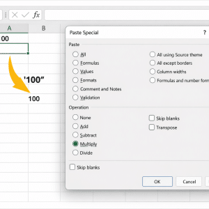
Method B: The “Multiply by 1” Trick

1. Type the number 1 in an empty cell.
2. Copy that cell.
3. Select your range of “text numbers.”
4. Right-click and choose Paste Special.
5. Select Multiply and click OK.
   Multiplying a text-number by 1 forces Excel to convert the result into a number.

---

Issue #2: The Dreaded “Ghost” Spaces

You are trying to sum sales for “Apple,” but your result is zero. You look at the cell, and it says “Apple.” What is going on?

Often, the cell actually contains “Apple ” (with a trailing space) or ” Apple” (with a leading space). Since “Apple” is not equal to “Apple “, your SUMIF formula is not working because the match isn’t exact.

The Problem

Trailing spaces are invisible. They often creep in during data entry or when copying data from websites. SUMIF requires an exact match for text criteria (unless you are using wildcards, which we will discuss later).

The Fix

You have two main options: clean the data or adjust the criteria.

Solution A: Clean the Source Data
Use the TRIM function to strip extra spaces.

1. Insert a helper column next to your data.
2. Use the formula =TRIM(A2) (assuming your data is in A2).
3. Copy this down for all rows.
4. Copy the new clean data and Paste Values over the original bad data.

Solution B: Use Wildcards in Your Formula
If you suspect spaces but can’t change the source data, use an asterisk * as a wildcard.
Instead of:
=SUMIF(A:A, "Apple", B:B)
Use:
=SUMIF(A:A, "*Apple*", B:B)

Note: This will also match “Pineapple” or “Crabapple,” so use with caution.

---

Issue #3: Mismatched Range Dimensions

This is a classic syntax error that can lead to incorrect totals without throwing an obvious error message. For SUMIF troubleshooting, checking range geometry is essential.

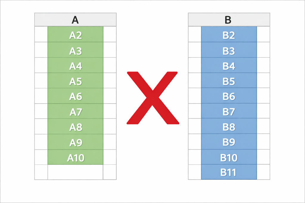
The Problem

The range (where you check criteria) and the sum_range (values to add) must be the same size and shape. If they aren’t, Excel behaves unpredictably.

Example of a mismatch:

• Range: A2:A100 (99 cells)
• Sum_range: B2:B105 (104 cells)

In older versions of Excel, the formula might automatically resize the sum_range to match the criteria range, but it shifts the cells, leading to summing the wrong rows. In newer dynamic array versions, this is less forgiving.

The Fix

Always ensure your start and end rows match exactly.

Incorrect:
=SUMIF(A2:A100, "East", B2:B200)

Correct:
=SUMIF(A2:A100, "East", B2:B100)

Pro Tip: Use Excel Tables (Ctrl+T). When you reference table columns (e.g., Table1[Region] and Table1[Sales]), Excel guarantees the ranges are the same size because a table always has consistent row counts.

---

Issue #4: Criterion Argument Syntax Errors

How you type your criteria matters immensely. Many users assume Excel understands logical context, but it requires specific syntax, especially when using comparison operators.

The Problem

You want to sum values greater than 50.
You type: =SUMIF(A:A, >50, B:B)
Result: Error popup. Excel thinks you are trying to start a formula incorrectly.

Or perhaps you want to reference a cell (C1) that contains the number 50.
You type: =SUMIF(A:A, ">C1", B:B)
Result: Zero. Excel is looking for the text string “>C1”, not the value inside cell C1.

The Fix

You must use quotation marks for operators and ampersands (&) for cell references.

Scenario A: Hardcoded Number
Correct syntax: =SUMIF(A:A, ">50", B:B)
The operator and number must be inside quotes.

Scenario B: Cell Reference
Correct syntax: =SUMIF(A:A, ">"&C1, B:B)
The operator goes in quotes, followed by an ampersand to join it with the cell reference.

Scenario C: Text Match
Correct syntax: =SUMIF(A:A, "London", B:B)
Text must always be in quotes.

---

Issue #5: Referring to Closed External Workbooks

You have a master summary sheet that pulls data from five different department spreadsheets. You write your SUMIFs, everything looks great. Then, you close the department spreadsheets, and suddenly your Excel formula is not working. Instead, you see #VALUE! errors.

The Problem

The SUMIF and SUMIFS functions do not work with closed workbooks. Unlike a simple VLOOKUP or a direct cell reference (=[Book1.xlsx]Sheet1!$A$1), SUMIF requires the source file to be open in memory to calculate. If the file is closed, the function breaks.

The Fix

This is an inherent limitation of SUMIF, but there are workarounds.

Solution A: Keep the Source Files Open
The simplest solution is to open the linked files whenever you need to update the summary.

Solution B: Use SUMPRODUCT Instead
The SUMPRODUCT function is more robust and can handle closed workbooks.
Instead of:
=SUMIF([Book1.xlsx]Sheet1!$A:$A, "Criteria", [Book1.xlsx]Sheet1!$B:$B)

Use:
=SUMPRODUCT(--([Book1.xlsx]Sheet1!$A:$A="Criteria"), [Book1.xlsx]Sheet1!$B:$B)

Note: SUMPRODUCT can be slower on very large datasets, but it solves the closed workbook error.

---

Issue #6: Hidden Characters and Non-Breaking Spaces

This is a level deeper than the “Ghost Spaces” issue. Sometimes you trim your data, remove extra spaces, and it still doesn’t work. You might be dealing with Non-Breaking Spaces (  in HTML), commonly found in data copied from web-based systems.

The Problem

A standard space character has an ASCII code of 32. A non-breaking space has an ASCII code of 160. The TRIM function only removes standard spaces (ASCII 32). To Excel, Char(160) is just another letter, not a space it can remove.

The Fix

You need to find and replace the specific character code.

Using Find & Replace:

1. Highlight your data column.
2. Press Ctrl + H to open Find & Replace.
3. In the “Find what” box, hold down Alt and type 0160 on your numeric keypad. (You won’t see anything appear, but it’s there).
4. Leave the “Replace with” box empty (or put a standard space if you want to keep the separation).
5. Click Replace All.

Using a Formula:
Use the SUBSTITUTE function combined with TRIM.
=TRIM(SUBSTITUTE(A2, CHAR(160), " "))
This replaces the non-breaking space with a regular space, then trims the result.

---

Issue #7: The Criteria Range Contains Errors

If the range you are evaluating contains errors like #N/A, #DIV/0!, or #VALUE!, SUMIF will often fail completely.

The Problem

SUMIF is generally robust enough to ignore errors in the sum_range (it just won’t sum that specific row), but errors in the criteria range can sometimes confuse the logic, especially if you are using complex criteria. Furthermore, if you are using SUMIFS (multiple criteria), a single error in any criteria column usually breaks the whole calculation.

The Fix

You need to clean the errors in your source data.

Solution A: Use IFERROR in Source Data
Go back to the formula generating your source data and wrap it in IFERROR.
=IFERROR(YourOriginalFormula, 0) or =IFERROR(YourOriginalFormula, "")

Solution B: Use AGGREGATE (Advanced)
If you cannot touch the source data, the AGGREGATE function is a powerful alternative that can be told specifically to ignore error values while summing.

=AGGREGATE(9, 6, Range)
(Note: AGGREGATE is more like a Subtotal function and works differently than SUMIF for conditional summing, but it is excellent for summing ranges with errors).

For conditional summing with errors, the best approach remains cleaning the source data using Solution A.

---

Summary Checklist: How to Fix SUMIF Formula

When your Excel formula is not working, run through this quick checklist:

1. Check Data Types: Are your numbers actually text? (Look for green triangles).
2. Inspect Spaces: Does ” Apple” match “Apple”? Try using wildcards.
3. Verify Ranges: Does the criteria range size match the sum range size?
4. Audit Syntax: Are you using quotes for operators (">100") and ampersands for cell refs (">"&A1)?
5. Check Source Files: Are you referencing a closed workbook? Switch to SUMPRODUCT.
6. Deep Clean: Are there hidden HTML spaces (Char 160)?
7. Error Check: Are there existing errors (#N/A) in the columns you are referencing?

---

Frequently Asked Questions (FAQ)

Q: Can SUMIF check two different criteria?
A: No, the standard SUMIF function handles only one condition. To check two or more criteria (e.g., “Sales” > 100 AND “Region” = “North”), you must use the SUMIFS function (note the “S” at the end).

Q: Is SUMIF case-sensitive?
A: No. SUMIF treats “apple”, “APPLE”, and “Apple” exactly the same. If you need a case-sensitive sum, you will need to use a SUMPRODUCT formula utilizing the EXACT function.

Q: Why does my SUMIF result update only when I press F9?
A: Your calculation options might be set to “Manual.” Go to the Formulas tab in the ribbon, click Calculation Options, and ensure it is set to Automatic.

Q: Can I use SUMIF with dates?
A: Yes! Dates in Excel are just serial numbers. You can use criteria like ">01/01/2023". However, it is safer to use the DATE function in your criteria to avoid regional format issues: =SUMIF(Range, ">"&DATE(2023,1,1), Sum_Range).

Q: How do I sum “not equal to” a specific value?
A: Use the <> operator. For example, to sum everything except “Red”, use <>"Red" as your criteria.

---

Test Your Knowledge: The SUMIF Troubleshooting Quiz

Think you’ve mastered the art of fixing SUMIF errors? Test your skills with this quick interactive quiz.

---

Conclusion

Excel formulas are logical, but they aren’t magical. When SUMIF is not working, it is almost always due to data inconsistency or syntax rules. By methodically checking for text-stored numbers, hidden spaces, and correct syntax, you can troubleshoot errors in minutes rather than hours.

Mastering these fixes doesn’t just repair your current spreadsheet—it makes you a better data analyst. You start to anticipate these issues before they happen, building cleaner, more robust models from day one.

So the next time you see that zero or #VALUE! error, don’t panic. Just run through the checklist, clean your data, and watch those numbers add up perfectly.