
1. What is Exploratory Data Analysis (EDA)?
Exploratory Data Analysis, commonly known as EDA, is the critical process of performing initial investigations on a dataset to discover patterns, spot anomalies, test hypotheses, and check assumptions — all with the help of summary statistics and graphical representations.
The term was popularized by the legendary statistician John W. Tukey in his 1977 book Exploratory Data Analysis. Tukey believed that data analysis should begin with open-ended exploration rather than immediately jumping to confirmatory statistical tests. His philosophy fundamentally reshaped how data scientists approach new datasets.
Think of EDA as a conversation with your data. You ask questions like: What does this column mean? Are there unusual values here? How are these two variables related? What surprises me about this distribution? The answers guide every decision you make during the modeling phase.
“Far better an approximate answer to the right question, which is often vague, than an exact answer to the wrong question.”— John W. Tukey, Statistician
EDA is not just about making pretty charts. It’s about building a deep, intuitive understanding of your data so that your modeling choices are grounded in reality rather than assumptions.
2. Why EDA Matters Before Modeling
Many beginners make the mistake of skipping EDA and jumping straight into machine learning. This leads to a cascade of problems that are difficult to debug later. Here’s why EDA is non-negotiable:
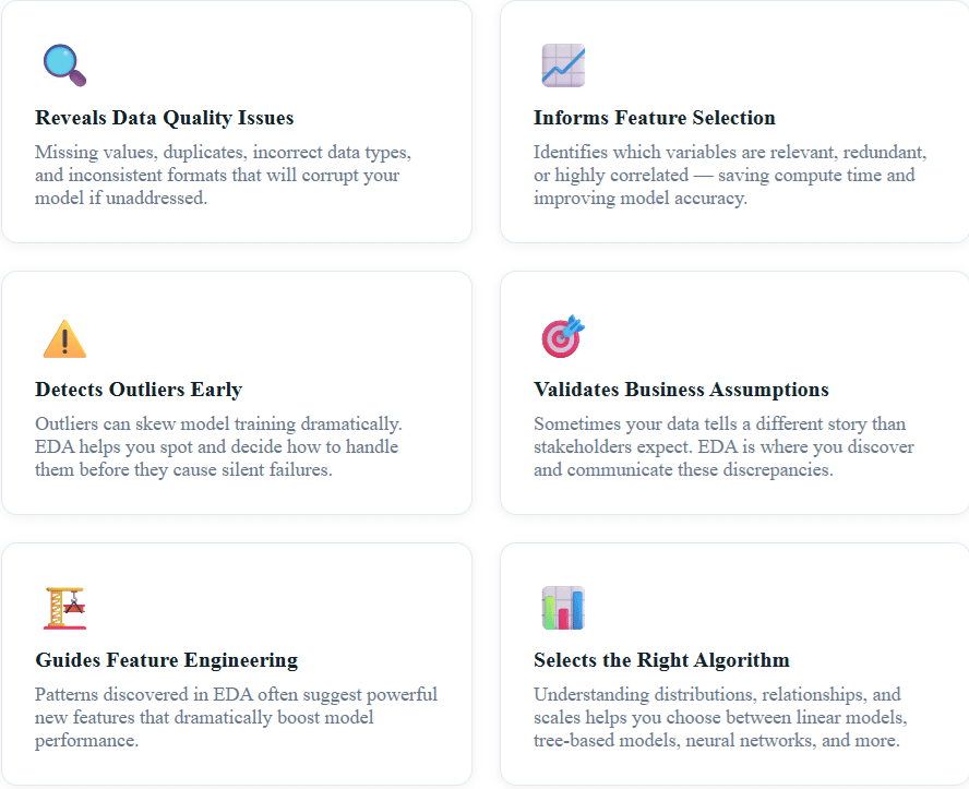
A 2020 survey by Kaggle found that data scientists spend nearly 45% of their project time on data understanding and preparation — more than any other phase. EDA is the most important investment you can make in a data science project.
3. The EDA Workflow: Step-by-Step
A structured EDA workflow prevents you from getting lost in a sea of plots and statistics. Here is the proven framework used by professional data scientists:
1
Data Collection & Loading — Load the data, understand its source, and verify it loaded correctly. Check shape, dtypes, and first few rows.
2
Data Overview & Structure — Examine data types, dimensions, column names, and basic descriptive statistics using df.info() and df.describe().
3
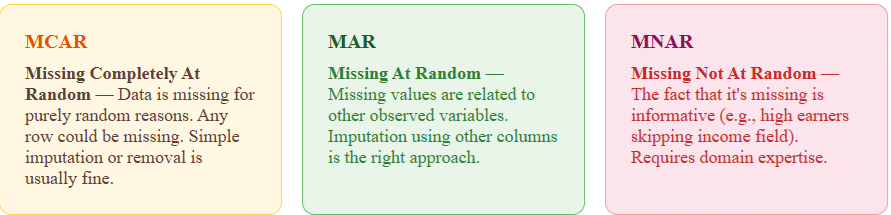
Missing Value Analysis — Quantify missing data per column, understand why it’s missing (MCAR, MAR, MNAR), and decide on imputation or removal strategies.
4
Univariate Analysis — Analyze each variable individually using histograms, box plots, and value counts to understand distributions.
5
Bivariate & Multivariate Analysis — Explore relationships between variables using scatter plots, correlation heatmaps, pair plots, and cross-tabulations.
6
Outlier Detection & Treatment — Identify statistical and domain-based outliers using IQR, Z-score, and visualization techniques.
7
Documentation & Insights Summary — Record all findings, surprising patterns, and decisions made. This becomes the foundation for your modeling strategy.
4. Univariate Analysis: Understanding Each Variable
Univariate analysis examines one variable at a time. The goal is to understand its distribution, central tendency, spread, and the presence of any unusual values. It’s your first deep dive into the data.
For Numerical Variables
The key statistics to examine for numerical variables are mean, median, mode, standard deviation, skewness, and kurtosis. Python’s Pandas makes this trivially easy:
import pandas as pd
import matplotlib.pyplot as plt
import seaborn as sns

# Load the Titanic dataset as an example
df = pd.read_csv('titanic.csv')

# Basic summary statistics
print(df.describe())

# Visualize age distribution
fig, axes = plt.subplots(1, 3, figsize=(15, 4))

df['Age'].hist(bins=30, ax=axes[0], color='#2c5364')
axes[0].set_title('Age Distribution')

df.boxplot(column='Age', ax=axes[1])
axes[1].set_title('Age Box Plot')

# Check skewness
print(f"Age Skewness: {df['Age'].skew():.2f}")
print(f"Age Kurtosis: {df['Age'].kurtosis():.2f}")
What to look for: A skewness value greater than 1 or less than -1 suggests significant skew — which may require log transformation before modeling. High kurtosis indicates heavy tails and potential outliers.
For Categorical Variables
For categorical columns, examine the frequency of each category, the number of unique values (cardinality), and watch for rare categories that may cause issues during train-test splits.
# Categorical analysis
print(df['Pclass'].value_counts())
print(df['Sex'].value_counts(normalize=True))  # proportions

# Bar chart for categorical column
df['Embarked'].value_counts().plot(kind='bar', color='#203a43')
plt.title('Embarkation Port Distribution')
plt.xticks(rotation=0)
plt.show()
5. Bivariate & Multivariate Analysis
While univariate analysis tells you about individual variables, bivariate and multivariate analysis reveals how variables interact with each other. This is where the real storytelling begins.
Correlation Analysis
The correlation matrix is one of the most powerful EDA tools. It shows the pairwise linear relationships between all numerical variables, instantly highlighting which features move together and which are redundant.
# Correlation Heatmap
plt.figure(figsize=(10, 8))
corr_matrix = df.select_dtypes(include='number').corr()

sns.heatmap(corr_matrix,
            annot=True,
            fmt='.2f',
            cmap='coolwarm',
            center=0,
            square=True)

plt.title('Feature Correlation Heatmap', fontsize=14)
plt.tight_layout()
plt.show()

# Find highly correlated pairs (threshold > 0.8)
high_corr = corr_matrix[corr_matrix > 0.8].stack()
high_corr = high_corr[high_corr.index.get_level_values(0) !=
                       high_corr.index.get_level_values(1)]
print("Highly correlated features:")
print(high_corr)
Key insight: If two features have a correlation above 0.85, you likely only need one of them. Keeping both introduces multicollinearity, which can destabilize models like Logistic Regression and Linear Regression.
Target Variable Analysis
Always analyze how each feature relates to your target variable. For classification problems, this might mean grouped bar charts or violin plots. For regression, scatter plots with trend lines are essential.
# Survival rate by passenger class (bivariate: categorical vs categorical)
survival_by_class = df.groupby('Pclass')['Survived'].mean()
survival_by_class.plot(kind='bar', color='#2c5364')
plt.title('Survival Rate by Passenger Class')
plt.ylabel('Survival Rate')
plt.show()

# Age vs Fare (numerical vs numerical) colored by target
plt.figure(figsize=(8, 6))
sns.scatterplot(data=df, x='Age', y='Fare',
                hue='Survived', alpha=0.6, palette='Set1')
plt.title('Age vs Fare colored by Survival')
plt.show()
6. Handling Missing Data: The Right Way
Missing data is one of the most common — and most consequential — data quality issues you’ll encounter. The strategy for handling it depends on why the data is missing.
# Analyze missing data
missing_data = df.isnull().sum()
missing_pct = (df.isnull().sum() / len(df)) * 100
missing_df = pd.DataFrame({
    'Missing Count': missing_data,
    'Missing Percentage': missing_pct
}).sort_values('Missing Percentage', ascending=False)

print(missing_df[missing_df['Missing Count'] > 0])

# Strategy: median imputation for Age (skewed distribution)
df['Age'].fillna(df['Age'].median(), inplace=True)

# Strategy: mode imputation for Embarked (categorical)
df['Embarked'].fillna(df['Embarked'].mode()[0], inplace=True)

# Strategy: drop Cabin (>77% missing, not recoverable)
df.drop(columns=['Cabin'], inplace=True)
Rule of thumb: If a column has more than 40% missing values and there’s no strong reason to impute, consider dropping it. If missing data itself carries signal (e.g., “Cabin number missing → likely 3rd class passenger”), create a binary indicator column before imputing.
7. Detecting and Treating Outliers
Outliers are data points that differ significantly from the overall pattern. They can be legitimate (a CEO’s salary in a workforce dataset), data errors (an age of 999), or important signals (fraudulent transactions). Context is everything.
Statistical Methods for Outlier Detection
The two most common statistical approaches are the IQR method and the Z-score method:
import numpy as np
from scipy import stats

# Method 1: IQR Method
Q1 = df['Fare'].quantile(0.25)
Q3 = df['Fare'].quantile(0.75)
IQR = Q3 - Q1

lower_bound = Q1 - 1.5 * IQR
upper_bound = Q3 + 1.5 * IQR

outliers_iqr = df[(df['Fare'] < lower_bound) | (df['Fare'] > upper_bound)]
print(f"IQR Outliers in Fare: {len(outliers_iqr)}")

# Method 2: Z-Score Method
z_scores = np.abs(stats.zscore(df['Fare'].dropna()))
outliers_z = df['Fare'].dropna()[z_scores > 3]
print(f"Z-Score Outliers in Fare: {len(outliers_z)}")

# Visualize with box plot
sns.boxplot(x=df['Fare'], color='#64ffda')
plt.title('Fare Distribution with Outliers')
plt.show()
Once detected, you have several options for treating outliers: removal (if they are errors), capping/winsorization (set values to the 1st/99th percentile), log transformation (reduces the impact of extreme values), or keeping them (if they carry real signal — especially in fraud detection).
8. Feature Engineering Inspired by EDA
The best features aren’t always the ones you start with. EDA often reveals hidden signals that can be encoded into powerful new features. This is where creativity and domain knowledge intersect.
Example: In the Titanic dataset, EDA might reveal that passengers with small families (2-4 members) had higher survival rates than solo travelers or large families. You could create a new FamilySize feature and then a categorical FamilyType feature:
# Feature engineering from EDA insights
df['FamilySize'] = df['SibSp'] + df['Parch'] + 1

def family_type(size):
    if size == 1:
        return 'Solo'
    elif size <= 4:
        return 'Small'
    else:
        return 'Large'

df['FamilyType'] = df['FamilySize'].apply(family_type)

# Verify the new feature's predictive power
survival_by_family = df.groupby('FamilyType')['Survived'].mean()
print(survival_by_family)
# Solo: 0.30, Small: 0.58, Large: 0.16 — great signal!
This kind of EDA-driven feature engineering is the reason experienced data scientists outperform beginners even when using the same algorithms. The features tell the story; the model just learns to read it.
9. Top EDA Tools and Libraries in 2024
The EDA ecosystem has evolved dramatically. You no longer need to write every visualization from scratch — here are the best tools available today:
| Tool / Library | Best For | Highlights |
|---|---|---|
| Pandas | Data wrangling & stats | describe(), info(), value_counts() |
| Seaborn | Statistical visualization | heatmaps, pair plots, violin plots |
| Plotly | Interactive visualizations | Zoom, hover, animated plots |
| ydata-profiling | Automated EDA reports | One-line comprehensive HTML report |
| Sweetviz | Comparative EDA | Train vs Test visualization |
| D-Tale | Interactive GUI EDA | No-code EDA interface in Jupyter |
| Tableau | Business stakeholder EDA | Drag-and-drop, shareable dashboards |
For rapid automated EDA, ydata-profiling (formerly pandas-profiling) is a game-changer. A single line of code generates a comprehensive HTML report with distributions, correlations, missing data analysis, and duplicate detection:
# Automated EDA with ydata-profiling
from ydata_profiling import ProfileReport

profile = ProfileReport(df, title="Titanic EDA Report", explorative=True)
profile.to_file("titanic_report.html")

# Or display inline in Jupyter
profile.to_notebook_iframe()
10. Real-World EDA Example: Housing Price Prediction
Let’s walk through a condensed real-world EDA using the Boston Housing dataset, which is a classic regression problem. This example shows how EDA directly informs modeling decisions.
Scenario: You’re building a model to predict house prices. You have 13 features including crime rate, number of rooms, distance to employment centers, and school quality metrics.
Step 1 — Load and Inspect: You run df.describe() and immediately notice that CRIM (crime rate) has a mean of 3.6 but a max of 88.9 — a massive right skew. This flags the need for log transformation.
Step 2 — Correlation Heatmap: The heatmap reveals that RM (average rooms per dwelling) has a strong positive correlation of 0.70 with the target variable MEDV (house price). Meanwhile, LSTAT (% lower status population) has a strong negative correlation of -0.74. These are your most predictive features.
Step 3 — Scatter Plots: Plotting RM vs MEDV reveals a linear relationship, but there’s a cluster of points capped at $50,000 — likely a data collection artifact where values above a threshold were capped. This would bias a regression model, and you decide to exclude these data points.
Step 4 — Distribution Analysis: MEDV itself shows a bimodal distribution — two peaks. This suggests there might be two distinct market segments in the data (affordable vs. premium housing), pointing toward either segment-based modeling or adding a neighborhood cluster feature.
Outcome of EDA: Before touching a model, you’ve identified the most important features, needed transformations (log for crime rate), a data quality issue (price capping), and a potential modeling strategy (market segmentation). This is the power of thorough EDA.
💡 Pro EDA Tips from Industry Practitioners
- Always look at your data manually (df.sample(20)) — automated tools miss context.
- Create an EDA document as you go. Your future self will thank you.
- Use log scale for heavily skewed financial data (sales, revenue, price).
- Plot distributions before and after transformations to verify improvement.
- Always split train/test before EDA to avoid data leakage into your test set.
- In time-series data, always plot the time dimension first — seasonality and trends change everything.
- Validate EDA findings with domain experts before proceeding to modeling.
Frequently Asked Questions (FAQ)
What is the difference between EDA and data preprocessing?
EDA is the investigative phase — you’re exploring data to understand its structure, patterns, and anomalies without yet making permanent changes. Data preprocessing is the transformation phase where you clean, encode, and scale the data based on what EDA revealed. EDA informs preprocessing decisions; preprocessing implements them. In practice, they often overlap, but conceptually EDA comes first.
How long should EDA take in a data science project?
There’s no fixed rule — it depends on dataset complexity, quality, and project requirements. As a rule of thumb, plan for EDA to take 20–30% of your total project time. For a fresh, complex dataset, EDA could take several days. For cleaner, familiar datasets you’ve worked with before, a few hours may suffice. Never rush EDA — time spent here saves multiples downstream.
Can I perform EDA on text or image data?
Absolutely. For text data, EDA involves analyzing word frequencies, text length distributions, vocabulary size, class imbalances, and using word clouds or TF-IDF visualizations. For image data, EDA includes checking image dimensions, color channel distributions, class balance, and viewing sample images per class. The principles of understanding your data before modeling apply universally.
What’s the best Python library for beginners doing EDA?
For absolute beginners, start with ydata-profiling for automated reports to see what EDA covers, then learn Pandas + Seaborn for manual exploration. Once comfortable, add Plotly for interactive plots. This progression builds understanding of what you’re computing, not just generating reports blindly.
Should I perform EDA on the full dataset or split first?
Always split your data into training and test sets before performing detailed EDA. If you explore the full dataset (including the test set) and use those insights to inform preprocessing decisions, you’ve introduced subtle data leakage. EDA should be performed on the training set only. You may look at the test set briefly to confirm it has the same structure, but not to derive statistical parameters used in transformations.
What is the difference between EDA and descriptive statistics?
Descriptive statistics are a component of EDA, not the whole picture. Descriptive statistics (mean, median, standard deviation, etc.) summarize numerical properties of the data. EDA is broader — it combines descriptive statistics with visualization, hypothesis generation, anomaly detection, and relationship exploration. EDA is as much an art as a science; descriptive statistics are purely mathematical.
How do I deal with class imbalance discovered during EDA?
Class imbalance (e.g., 95% “No Fraud”, 5% “Fraud”) is critical to discover during EDA. Treatment options include: oversampling the minority class (SMOTE), undersampling the majority class, using class weights in your model, or choosing evaluation metrics that handle imbalance well (F1-score, AUC-ROC instead of accuracy). The right choice depends on the cost of different error types in your specific domain.