1. What is the SUMIF Function in Excel?
The SUMIF function in Excel is one of the most powerful and widely used formulas for data analysis. It allows you to sum values in a range based on a specific condition or criteria — meaning Excel will only add up the numbers that meet your specified requirement.
Think of SUMIF as a smarter version of the basic SUM function. While SUM blindly adds everything, SUMIF is selective — it only totals the values that satisfy your condition.
💡Real-World Analogy
Imagine you have a grocery receipt with 50 items. Instead of adding every item, you want to know: “How much did I spend on vegetables only?” SUMIF does exactly this — it scans the “category” column, finds all “Vegetable” entries, and sums only their prices.
SUMIF was introduced in Excel 97 and has been a staple of data analysis ever since. It belongs to the family of conditional aggregation functions, alongside COUNTIF, AVERAGEIF, SUMIFS, and others.
When Should You Use SUMIF?
You should use SUMIF when you need to:
- Calculate total sales for a specific product, region, or salesperson
- Sum expenses within a specific category (food, travel, utilities)
- Add up values that are greater than or less than a threshold
- Total transactions before or after a specific date
- Aggregate data from large datasets based on any matching condition
2. SUMIF Syntax Explained
Understanding the SUMIF syntax is the foundation of using it effectively. The function takes three arguments — two required and one optional.

Breaking Down Each Argument
Argument 1: range (Required)
The range is the group of cells that Excel will evaluate against your criteria. This is the column or row that Excel “scans” to look for matches. For example, if you want to sum sales by region, your range would be the “Region” column.
Argument 2: criteria (Required)
The criteria is the condition that must be met for a value to be included in the sum. It can be:
| Criteria Type | Example | Description |
|---|---|---|
| Text (exact match) | "North" | Matches cells containing exactly “North” |
| Number | 100 | Matches cells equal to 100 |
| Comparison | ">500" | Matches cells greater than 500 |
| Wildcard | "Ap*" | Matches any text starting with “Ap” |
| Cell Reference | A2 | Matches whatever value is in cell A2 |
| Date | ">"&DATE(2024,1,1) | Matches dates after Jan 1, 2024 |
Argument 3: sum_range (Optional)
The sum_range is the range of cells that Excel will actually add up when a match is found in the range. If omitted, Excel sums the values in the range itself.
⚠️Important Note
The
rangeandsum_rangemust be the same size (same number of rows and columns). If they differ, Excel uses the top-left cell ofsum_rangeas the starting point and expands to matchrange.
3. Basic SUMIF Examples
Let’s start with a practical dataset. Suppose you have a sales table for a retail store:
| A — Product | B — Region | C — Salesperson | D — Sales ($) |
|---|---|---|---|
| Laptop | North | Alice | 1200 |
| Phone | South | Bob | 800 |
| Laptop | East | Alice | 1500 |
| Tablet | North | Carol | 600 |
| Phone | North | Bob | 900 |
| Laptop | South | Carol | 1100 |
| Tablet | East | Alice | 700 |
| Total Laptop Sales | ? | ||
EXAMPLE 1 : Sum sales for “Laptop” only
=SUMIF(A2:A8, “Laptop”, D2:D8) // Result: 3800 (1200 + 1500 + 1100)
How it works: Excel looks through
A2:A8, finds every cell that says “Laptop”, then adds up the corresponding values fromD2:D8.
EXAMPLE 2 : Sum sales for “North” region
=SUMIF(B2:B8, “North”, D2:D8) // Result: 2700 (1200 + 600 + 900)
How it works: Excel scans column B for “North” and sums matching values from column D.
EXAMPLE 3 : Using a cell reference as criteria
=SUMIF(C2:C8, F2, D2:D8) // Where F2 contains “Alice” // Result: 3400 (1200 + 1500 + 700)
Using a cell reference makes your formula dynamic — just change the value in F2 and the sum updates automatically. This is ideal for dashboards and reports.
4. SUMIF with Text Criteria
Text criteria in SUMIF are case-insensitive by default. “laptop”, “LAPTOP”, and “Laptop” are all treated as identical. Here are the most important text-based SUMIF patterns:
Exact Text Match
=SUMIF(A2:A100, “Laptop”, D2:D100) // Sums only exact matches of “Laptop”
Not Equal to Text
Use the <> operator to sum everything except a specific text value:
=SUMIF(A2:A100, “<>Laptop”, D2:D100) // Sums all rows where product is NOT “Laptop”
Text Containing a Word (Partial Match)
=SUMIF(A2:A100, “*Pro*”, D2:D100) // Sums rows where product name contains “Pro” anywhere // Matches: “MacBook Pro”, “Pro Plus”, “ProMax”, etc.
⭐Pro Tip: Concatenate Cell Reference with Wildcard
=SUMIF(A2:A100, "*"&F2&"*", D2:D100)— This combines a wildcard with a cell reference, creating a dynamic partial match formula that’s perfect for search-style dashboards.
5. SUMIF with Number and Comparison Criteria
SUMIF becomes incredibly powerful when you combine it with comparison operators. These must always be enclosed in double quotes when hard-coded.
| Operator | Meaning | Example Formula | What It Does |
|---|---|---|---|
> | Greater than | =SUMIF(D2:D100,">1000",D2:D100) | Sums values over 1000 |
< | Less than | =SUMIF(D2:D100,"<500",D2:D100) | Sums values under 500 |
>= | Greater than or equal | =SUMIF(D2:D100,">=1000",D2:D100) | Sums values 1000 or more |
<= | Less than or equal | =SUMIF(D2:D100,"<=500",D2:D100) | Sums values 500 or less |
= | Equals | =SUMIF(D2:D100,1000,D2:D100) | Sums values exactly 1000 |
<> | Not equal | =SUMIF(D2:D100,"<>0",D2:D100) | Sums all non-zero values |
Using Cell References in Comparison Criteria
When your threshold value is in a cell, you need to concatenate the operator with the cell reference using the & symbol:
=SUMIF(D2:D100, “>”&G1, D2:D100) // Where G1 contains your threshold value (e.g. 1000) // This is DYNAMIC — change G1 and the result updates instantly
REAL WORLD Budget Analysis — Sum Over-Budget Expenses
=SUMIF(C2:C50, “>”&Budget_Limit, C2:C50) // Sums all expense entries that exceed the budget limit // Useful for flagging overspending categories
This formula is commonly used in financial tracking to instantly identify how much over-budget spending has occurred across all categories.
6. SUMIF with Wildcards (* and ?)
Wildcards are special characters that represent unknown or variable text — they unlock fuzzy or partial matching in SUMIF.
| Wildcard | Meaning | Example | Matches |
|---|---|---|---|
* | Zero or more characters | "Apple*" | Apple, Apple Pro, AppleMax |
* | At end = ends with | "*book" | Notebook, Macbook, Textbook |
* | Both sides = contains | "*mini*" | Mini Tablet, Pro mini, mini2 |
? | Exactly one character | "M?n" | Man, Men, Min, Mon |
~* | Literal asterisk | "Price~*" | Only cells containing “Price*” |
EXAMPLE : Sum all iPhone model sales
=SUMIF(A2:A200, “iPhone*”, B2:B200) // Matches: iPhone 14, iPhone 15 Pro, iPhone SE, iPhone Max… // Doesn’t match: Samsung, iPad, MacBook
This is especially useful when product names follow a naming convention where the brand or category is always at the start or end.
7. SUMIF with Dates
Working with dates in SUMIF requires special care. Excel stores dates as serial numbers, so comparisons work, but you need the right syntax.
Sum Values Before / After a Specific Date
=SUMIF(B2:B100, “<“&DATE(2024,7,1), C2:C100) // Sums sales before July 1, 2024
=SUMIF(B2:B100, “>=”&DATE(2024,1,1), C2:C100) // Sums sales from Jan 1, 2024 onwards
Sum for a Specific Year Using SUMPRODUCT + YEAR
=SUMPRODUCT((YEAR(B2:B100)=2024)*C2:C100) // Alternative to SUMIF for year-based filtering
Sum for Current Month (Dynamic)
=SUMIFS(C2:C100, B2:B100, “>=”&EOMONTH(TODAY(),-1)+1, B2:B100, “<=”&EOMONTH(TODAY(),0)) // Sums values in the current calendar month (updates automatically)
📅Always Use DATE() for Hard-Coded Dates
Instead of writing
">01/07/2024"(which can misinterpret date formats), always use theDATE(year, month, day)function. This ensures cross-region compatibility.
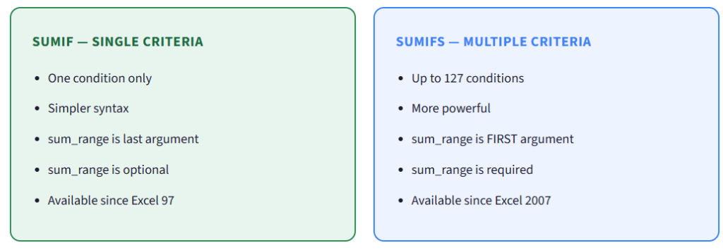
8. SUMIF vs SUMIFS: Multiple Criteria
When you need to filter by more than one condition simultaneously, you need SUMIFS — the plural, multi-criteria version of SUMIF.
SUMIFS Syntax
=SUMIFS(sum_range, criteria_range1, criteria1, [criteria_range2, criteria2], …) // NOTE: sum_range comes FIRST in SUMIFS (opposite of SUMIF)
SUMIFS EXAMPLE : Total Laptop sales in the North region by Alice
=SUMIFS(D2:D8, A2:A8, “Laptop”, B2:B8, “North”, C2:C8, “Alice”) // Three conditions: Product = Laptop AND Region = North AND Salesperson = Alice
All conditions in SUMIFS work with AND logic — meaning all conditions must be true simultaneously for a row to be included in the sum.
⚠️Common Mistake: Argument Order The #1 error people make switching from SUMIF to SUMIFS is forgetting that
sum_rangeis the first argument in SUMIFS, not the last.SUMIF:
=SUMIF(range, criteria, sum_range)
SUMIFS:=SUMIFS(sum_range, range1, criteria1, ...)
9. Advanced SUMIF Techniques
Technique 1: SUMIF Across Multiple Columns (Array Formula)
To sum across multiple criteria ranges simultaneously with OR logic:
=SUMPRODUCT(SUMIF(A2:A100, {“Laptop”,”Tablet”}, D2:D100)) // Sums sales for EITHER Laptop OR Tablet (OR logic) // No Ctrl+Shift+Enter needed — works as a regular formula
Technique 2: SUMIF in a Different Sheet
Reference data from another worksheet by including the sheet name:
=SUMIF(Sales!A:A, “Laptop”, Sales!D:D) // Sums Laptop sales from the “Sales” worksheet =SUMIF(‘[SalesData.xlsx]Sheet1’!A:A, “Laptop”, ‘[SalesData.xlsx]Sheet1’!D:D) // From an external workbook (must be open)
Technique 3: Dynamic SUMIF Dashboard (with Dropdown)
=SUMIF(B:B, H1, D:D) // H1 has a Data Validation dropdown list of regions // Selecting any region instantly updates the total // Perfect for executive dashboards and reports
Technique 4: Nested SUMIF for Tiered Analysis
=SUMIF(D2:D100,”>1000″,D2:D100) – SUMIF(D2:D100,”>5000″,D2:D100) // Sums values between 1000 and 5000 (mid-tier range) // Tip: For cleaner range summing, use SUMIFS instead
🎯 Performance Tip for Large Datasets
For datasets with 100,000+ rows, avoid using entire column references like
A:A. Instead, useA2:A100000. Using whole-column references forces Excel to calculate every cell, slowing down your workbook significantly.
.
10. Common SUMIF Errors and How to Fix Them
| Error | Common Cause | Fix |
|---|---|---|
| #VALUE! | Criteria entered incorrectly; comparison operator not in quotes | Wrap operator in quotes: ">100" not >100 |
| #NAME? | Misspelled function name; SUMIF typed as SUMIF (typo) | Check spelling; ensure no extra spaces in function name |
| 0 result | Text formatted as numbers, or leading/trailing spaces in data | Use TRIM() to clean data; check cell format (Text vs Number) |
| Wrong total | Range and sum_range sizes don’t match | Ensure both ranges cover exactly the same number of rows |
| #REF! | Range was deleted or formula points to invalid range | Re-enter the formula with correct cell references |
Debugging Tip: Use COUNTIF First
If your SUMIF returns 0 unexpectedly, first run a COUNTIF with the same range and criteria. If COUNTIF also returns 0, the issue is in how your data is stored (text vs numbers, spaces, etc.). If COUNTIF finds matches but SUMIF returns 0, the issue is with the sum_range.
=COUNTIF(A2:A100, “Laptop”) // If this returns 0, your data has a formatting or spacing issue // Fix the source data before trying SUMIF again
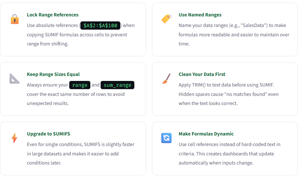
11. Pro Tips & Best Practices
Test Your SUMIF Knowledge!
7 questions • Excel SUMIF Function Quiz • Score: 1 point each
Quiz Complete!
12. Frequently Asked Questions (FAQ)
Can SUMIF handle case-sensitive matching?
No — SUMIF is inherently case-insensitive. “apple”, “Apple”, and “APPLE” are all treated as identical. If you need case-sensitive summing, use an array formula: =SUMPRODUCT((EXACT(A2:A100,"Apple"))*B2:B100) — this uses the EXACT() function which IS case-sensitive.
What is the maximum number of characters in SUMIF criteria?
The criteria argument in SUMIF can be up to 255 characters long. If you need to match longer text strings, consider restructuring your data or using a helper column with a shorter identifier.
Can SUMIF work with OR logic (sum if A or B)?
SUMIF itself uses exact single-condition matching, but you can achieve OR logic by adding multiple SUMIF results: =SUMIF(A:A,"Laptop",D:D)+SUMIF(A:A,"Tablet",D:D). Alternatively, use: =SUMPRODUCT(SUMIF(A:A,{"Laptop","Tablet"},D:D)) for a cleaner approach.
Does SUMIF work with blank or empty cells?
Yes! Use =SUMIF(A2:A100,"",B2:B100) to sum values where the criteria range is blank. Use =SUMIF(A2:A100,"<>",B2:B100) to sum values where the criteria range is NOT blank. This is useful for handling missing data.
Why does my SUMIF return a different value than expected?
The most common causes are: (1) Numbers stored as text in the criteria range, (2) Leading or trailing spaces in cells — use TRIM() to clean, (3) Mismatched range sizes between range and sum_range, (4) Date format issues — use the DATE() function for dates, (5) The criteria contains extra characters or wrong spelling.
Can I use SUMIF with a pivot table?
Technically yes, but it’s unusual and not recommended. Pivot Tables have built-in aggregation tools that are far more efficient. However, you can write SUMIF formulas that reference cells in a pivot table’s output range — just be aware that if the pivot table layout changes, your SUMIF references may break.
What’s the difference between SUMIF and SUMPRODUCT?
SUMIF is specifically designed for conditional summing with a simple syntax, while SUMPRODUCT is a general-purpose function that multiplies arrays and sums the results. SUMPRODUCT is more flexible (handles complex conditions, case-sensitivity, multiple arrays) but slower for simple tasks. For straightforward conditional sums, SUMIF is faster and easier to read. Use SUMPRODUCT when SUMIF/SUMIFS can’t achieve what you need.
Can SUMIF reference another Excel workbook?
Yes. You can reference data from another workbook, but that workbook must be open for the formula to recalculate. Syntax: =SUMIF('[WorkbookName.xlsx]SheetName'!A:A,"Criteria",'[WorkbookName.xlsx]SheetName'!D:D). For better reliability, consider copying data locally or using Power Query to import external data.
Conclusion
The SUMIF function in Excel is an essential tool for anyone working with data. Whether you’re summing sales by product, calculating expenses by category, or building dynamic dashboards, SUMIF gives you the power to extract meaningful insights from raw data in seconds.
Start with the basic single-criteria SUMIF, then graduate to SUMIFS for multiple conditions. Combine wildcards for flexible matching, use cell references for dynamic formulas, and always clean your data to avoid frustrating zero-results. With the techniques covered in this guide, you’re equipped to handle virtually any conditional summing challenge in Excel.
🚀 What to Learn Next
Now that you’ve mastered SUMIF, explore: COUNTIF & COUNTIFS (conditional counting), AVERAGEIF & AVERAGEIFS (conditional averaging), XLOOKUP (modern replacement for VLOOKUP), and Power Query (for transforming large datasets without formulas).