How to handle imbalanced datasets in Python: Strategies and Solutions

Introduction: How to handle Imbalanced Datasets

In the realm of machine learning and data science, imbalanced datasets represent one of the most common yet challenging obstacles practitioners face. An imbalanced dataset occurs when the distribution of classes in your training data is heavily skewed, with one class significantly outnumbering others. This disparity can severely impact model performance, leading to biased predictions and unreliable results.

Imagine training a fraud detection system where only 0.1% of transactions are fraudulent. A naive model could achieve 99.9% accuracy simply by predicting “not fraud” for every transaction—yet it would fail entirely at its intended purpose. This scenario illustrates why understanding and addressing class imbalance is critical for building effective machine learning solutions.

In this comprehensive guide, we’ll explore proven strategies and solutions for dealing with imbalanced datasets, from fundamental resampling techniques to advanced algorithmic approaches. Whether you’re working on fraud detection, medical diagnosis, anomaly detection, or customer churn prediction, these techniques will help you build more robust and reliable models.

---

What Are Imbalanced Datasets?

Defining Class Imbalance

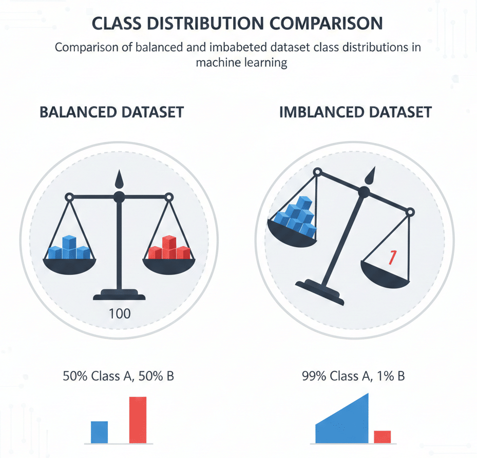
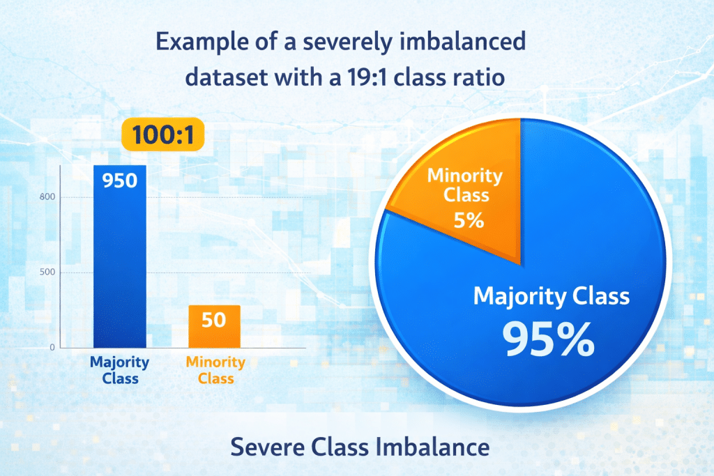
An imbalanced dataset is characterized by a significant disproportion in the number of samples across different classes. In binary classification problems, this typically means one class (the majority class) has substantially more samples than the other (the minority class). The imbalance ratio can range from moderate (4:1) to extreme (1000:1 or higher).

Types of Imbalance

Binary Class Imbalance:

• Two classes with unequal distribution
• Common in fraud detection, disease diagnosis
• Example: 95% negative samples, 5% positive samples

Multi-class Imbalance:

• Multiple classes with varying sample sizes
• Some classes may be severely underrepresented
• Example: Image classification with rare categories

Multi-label Imbalance:

• Samples can belong to multiple classes simultaneously
• Each label may have different prevalence rates
• Example: Document categorization, medical coding

Real-World Examples

Imbalanced datasets appear across numerous domains:

1. Fraud Detection: Financial transactions where fraudulent cases represent less than 1% of total transactions
2. Medical Diagnosis: Disease screening where positive cases are rare (cancer detection, rare genetic disorders)
3. Customer Churn: Predicting which customers will leave a service (typically 5-20% churn rate)
4. Manufacturing Defects: Quality control where defective products are uncommon
5. Spam Detection: Email filtering where spam may constitute 10-30% of messages
6. Network Security: Intrusion detection where attacks are infrequent
7. Credit Risk Assessment: Loan default prediction where defaults occur in 2-5% of cases

---

Why Imbalanced Datasets Pose Problems

The Accuracy Paradox

Traditional accuracy metrics become misleading with imbalanced data. Consider a dataset with 99% negative and 1% positive samples. A model that always predicts negative achieves 99% accuracy but identifies zero positive cases—rendering it useless for practical applications.

This accuracy paradox demonstrates why standard evaluation metrics fail with imbalanced datasets. The model appears successful by traditional measures while completely failing at its primary objective.

Bias Toward Majority Class

Machine learning algorithms typically optimize for overall accuracy, causing them to develop a strong bias toward the majority class. This occurs because:

1. Loss Function Optimization: Standard loss functions weight all errors equally, making majority class errors more impactful on total loss
2. Decision Boundary Skewing: The optimal decision boundary shifts toward the minority class region
3. Feature Importance Distortion: Features distinguishing minority class samples may be undervalued

Poor Minority Class Prediction

The consequences of majority class bias include:

• Low Recall: The model fails to identify most minority class instances
• High False Negative Rate: Many positive cases are incorrectly classified as negative
• Missed Critical Cases: In applications like medical diagnosis, failing to identify positive cases can have severe consequences
• Overfitting to Majority Patterns: The model learns to recognize majority class patterns while ignoring minority class characteristics

Impact on Different Algorithms

Various algorithms respond differently to class imbalance:

Decision Trees:

• Tend to favor splits that benefit the majority class
• May create shallow trees that ignore minority class patterns
• Can be highly biased without proper handling

Neural Networks:

• Often converge to solutions that prioritize majority class
• May require careful loss function design
• Benefit from balanced mini-batches during training

Support Vector Machines (SVM):

• Default formulation may place decision boundary suboptimally
• Can be improved with class weights
• Sensitive to kernel choice with imbalanced data

Ensemble Methods:

• Random Forests may create trees biased toward majority class
• Boosting algorithms can adapt better with proper configuration
• Benefit from balanced sampling strategies

---

Evaluation Metrics for Imbalanced Datasets

Beyond Accuracy: Better Metrics

When working with imbalanced datasets, selecting appropriate evaluation metrics is crucial. Here are the most effective alternatives:

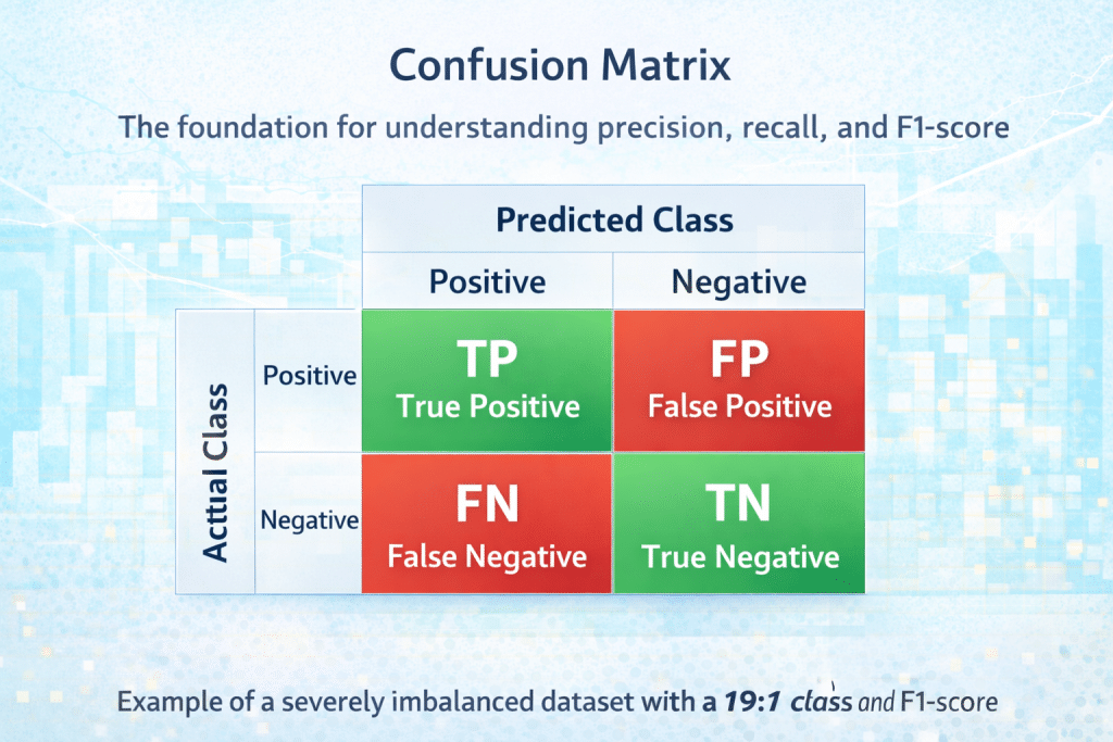
Confusion Matrix: A confusion matrix provides a complete picture of classifier performance:

                Predicted Negative    Predicted Positive
Actual Negative        TN                    FP
Actual Positive        FN                    TP

Where:

• True Negative (TN): Correctly predicted negative cases
• True Positive (TP): Correctly predicted positive cases
• False Negative (FN): Positive cases incorrectly predicted as negative
• False Positive (FP): Negative cases incorrectly predicted as positive

Precision: Precision = TP / (TP + FP)

Precision measures the proportion of positive predictions that are actually correct. High precision means few false positives. Critical when the cost of false positives is high (e.g., spam filtering).

Recall (Sensitivity): Recall = TP / (TP + FN)

Recall measures the proportion of actual positive cases correctly identified. High recall means few false negatives. Essential when missing positive cases is costly (e.g., cancer detection).

F1-Score: F1 = 2 × (Precision × Recall) / (Precision + Recall)

The F1-score provides a balanced measure combining precision and recall. It’s particularly useful when you need to balance both metrics equally.

F-Beta Score: F-Beta allows weighting precision or recall based on application requirements:

• F2-Score: Weights recall higher than precision
• F0.5-Score: Weights precision higher than recall

Matthews Correlation Coefficient (MCC): MCC = (TP×TN – FP×FN) / √[(TP+FP)(TP+FN)(TN+FP)(TN+FN)]

MCC ranges from -1 to +1, where +1 indicates perfect prediction, 0 indicates random prediction, and -1 indicates complete disagreement. It’s considered one of the most informative metrics for imbalanced datasets.

Area Under ROC Curve (AUC-ROC): The ROC curve plots True Positive Rate against False Positive Rate at various classification thresholds. AUC-ROC summarizes this relationship in a single number (0.5 = random, 1.0 = perfect).

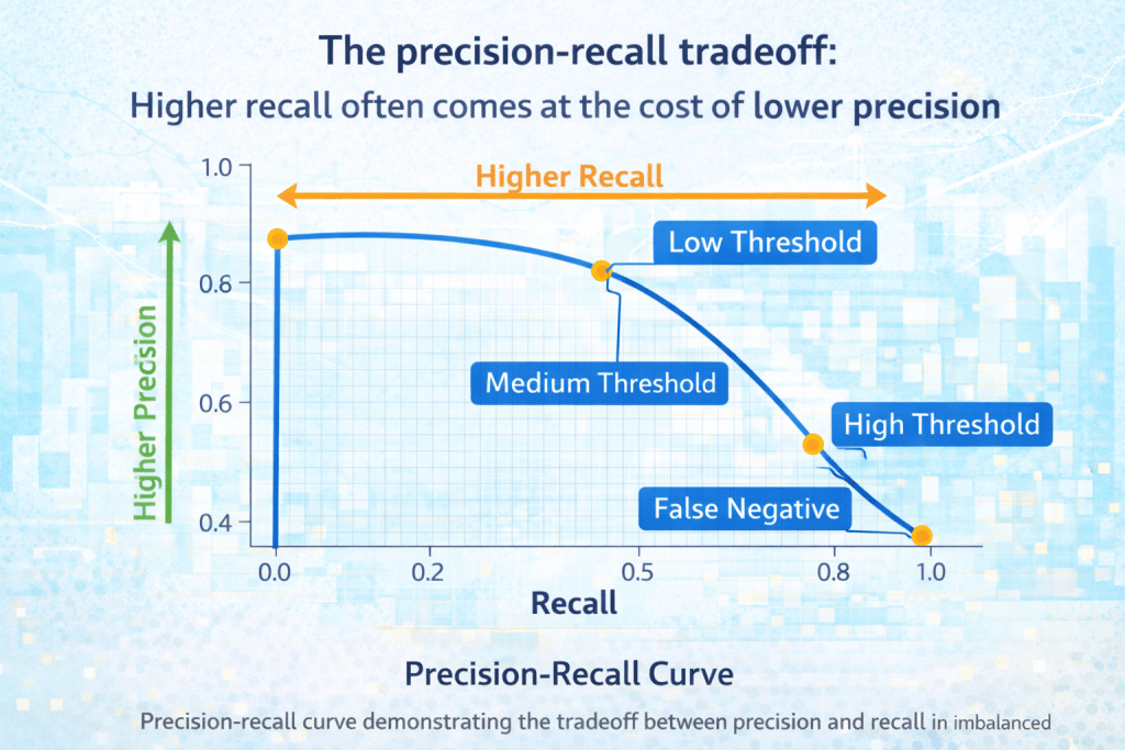
Precision-Recall Curve and AUC-PR: For severely imbalanced datasets, the Precision-Recall curve often provides more insight than ROC curves. The Area Under the Precision-Recall Curve (AUC-PR) is particularly informative when positive class is rare.

Choosing the Right Metric

Select metrics based on your application requirements:

Use Precision when:

• False positives are costly
• You need high confidence in positive predictions
• Example: Email spam detection (users tolerate some spam but hate losing legitimate emails)

Use Recall when:

• False negatives are costly
• You must identify most positive cases
• Example: Cancer screening (missing a case is worse than a false alarm)

Use F1-Score when:

• You need balanced precision and recall
• Both false positives and false negatives have similar costs
• Example: General classification tasks with moderate imbalance

Use MCC when:

• You want a single, balanced metric
• Dataset is highly imbalanced
• Example: Comprehensive model comparison

Use AUC-PR when:

• Dataset is severely imbalanced
• You want threshold-independent evaluation
• Example: Fraud detection with extreme imbalance

---

Resampling Techniques

Resampling methods modify the training dataset to balance class distribution. These are among the most straightforward and effective techniques for handling imbalanced data.

Random Oversampling

Concept: Random oversampling duplicates minority class samples randomly until classes are balanced or reach a desired ratio.

How It Works:

1. Identify minority class samples
2. Randomly select samples with replacement
3. Add copies to the training set
4. Repeat until target balance is achieved

Advantages:

• Simple to implement
• No information loss from majority class
• Works with any classifier
• Computationally inexpensive

Disadvantages:

• Risk of overfitting (model memorizes duplicated samples)
• Doesn’t add new information
• Can increase training time
• May amplify noise in minority class

Implementation Example (Python):

python

from imblearn.over_sampling import RandomOverSampler
from sklearn.datasets import make_classification

# Create imbalanced dataset
X, y = make_classification(n_samples=1000, n_classes=2, 
                          weights=[0.9, 0.1], random_state=42)

# Apply random oversampling
ros = RandomOverSampler(random_state=42)
X_resampled, y_resampled = ros.fit_resample(X, y)

print(f"Original class distribution: {Counter(y)}")
print(f"Resampled class distribution: {Counter(y_resampled)}")

Best Practices:

• Use with cross-validation to detect overfitting
• Combine with ensemble methods for better generalization
• Consider partial oversampling (e.g., 70% balance) rather than complete balance
• Monitor validation performance carefully

Random Undersampling

Concept: Random undersampling removes majority class samples randomly until classes are balanced.

How It Works:

1. Identify majority class samples
2. Randomly select subset of majority samples to keep
3. Remove remaining majority samples
4. Result: balanced or desired class ratio

Advantages:

• Reduces dataset size and training time
• Simple to implement
• No risk of overfitting minority class
• Can improve computational efficiency

Disadvantages:

• Loss of potentially valuable information
• May remove important majority class patterns
• Can lead to underfitting
• Sampling variance may affect results

Implementation Example:

python

from imblearn.under_sampling import RandomUnderSampler

# Apply random undersampling
rus = RandomUnderSampler(random_state=42)
X_resampled, y_resampled = rus.fit_resample(X, y)

print(f"Original class distribution: {Counter(y)}")
print(f"Resampled class distribution: {Counter(y_resampled)}")

Best Practices:

• Use when you have abundant majority class data
• Consider ensemble undersampling (EasyEnsemble)
• Maintain representative sample of majority class
• Validate that removed samples don’t contain critical patterns

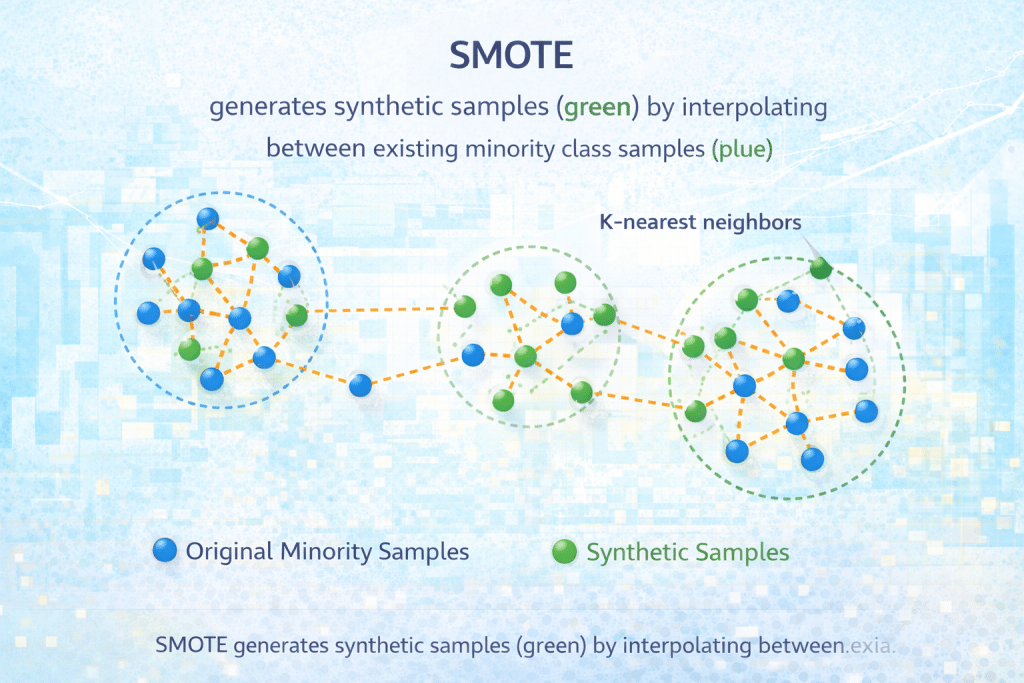
SMOTE (Synthetic Minority Over-sampling Technique)

Concept: SMOTE creates synthetic minority class samples by interpolating between existing minority samples, rather than duplicating them.

How It Works:

1. Select a minority class sample
2. Find its k-nearest minority class neighbors (typically k=5)
3. Choose one neighbor randomly
4. Create synthetic sample along the line segment between the two samples
5. Repeat until desired balance is achieved

Mathematical Formula:

synthetic_sample = original_sample + λ × (neighbor_sample - original_sample)

where λ is a random number between 0 and 1

Advantages:

• Generates new, diverse samples
• Reduces overfitting risk compared to simple oversampling
• Creates decision boundaries more representative of minority class
• No information loss from majority class

Disadvantages:

• Can generate noisy samples in overlapping regions
• Computationally more expensive than random sampling
• May create synthetic samples in wrong feature space
• Requires careful parameter tuning (k-neighbors)

Implementation Example:

python

from imblearn.over_sampling import SMOTE

# Apply SMOTE
smote = SMOTE(k_neighbors=5, random_state=42)
X_resampled, y_resampled = smote.fit_resample(X, y)

print(f"Original class distribution: {Counter(y)}")
print(f"Resampled class distribution: {Counter(y_resampled)}")

Variants:

• Borderline-SMOTE: Focuses on samples near decision boundary
• ADASYN: Adaptive Synthetic Sampling – generates more samples in harder-to-learn regions
• SMOTE-NC: For datasets with categorical features
• SMOTE-N: For purely categorical features

Best Practices:

• Apply SMOTE only to training data, never test data
• Experiment with k-neighbors parameter (typically 3-7)
• Consider borderline-SMOTE for cleaner synthetic samples
• Combine with undersampling for optimal results (SMOTE-ENN, SMOTE-Tomek)

Tomek Links

Concept: Tomek Links identifies pairs of samples from different classes that are each other’s nearest neighbors and removes the majority class sample from each pair. This cleans the decision boundary.

How It Works:

1. For each sample pair (sample_i, sample_j) from different classes
2. Check if they are each other’s nearest neighbors
3. If yes, they form a Tomek Link
4. Remove the majority class sample from the pair

Advantages:

• Cleans overlapping regions
• Improves decision boundary clarity
• Can be combined with oversampling
• Removes potentially noisy samples

Disadvantages:

• Only removes borderline cases
• May not significantly change class distribution
• Computationally expensive for large datasets

Implementation Example:

python

from imblearn.under_sampling import TomekLinks

# Apply Tomek Links
tomek = TomekLinks()
X_resampled, y_resampled = tomek.fit_resample(X, y)

Combined Resampling: SMOTE + Tomek Links

Concept: This hybrid approach first applies SMOTE to create synthetic minority samples, then uses Tomek Links to clean the decision boundary.

Advantages:

• Balances classes while cleaning boundaries
• Reduces noise from SMOTE
• Often achieves better performance than either technique alone

Implementation Example:

python

from imblearn.combine import SMOTETomek

# Apply SMOTE + Tomek Links
smote_tomek = SMOTETomek(random_state=42)
X_resampled, y_resampled = smote_tomek.fit_resample(X, y)

---

Algorithmic Approaches

Beyond resampling, several algorithmic techniques can effectively handle imbalanced datasets by modifying how models learn.

Class Weight Adjustment

Concept: Assign higher weights to minority class samples during training, making errors on these samples more costly and encouraging the model to pay more attention to them.

How It Works: The loss function is modified to incorporate class weights:

Weighted_Loss = Σ(weight_i × loss_i)

For imbalanced datasets, minority class weight is set proportionally higher:

weight_minority = n_samples / (n_classes × n_minority_samples)
weight_majority = n_samples / (n_classes × n_majority_samples)

Implementation Examples:

Scikit-learn (Logistic Regression, SVM, Random Forest):

python

from sklearn.linear_model import LogisticRegression
from sklearn.ensemble import RandomForestClassifier

# Automatic class weight balancing
lr = LogisticRegression(class_weight='balanced')
rf = RandomForestClassifier(class_weight='balanced')

# Manual class weights
class_weights = {0: 1, 1: 10}  # Weight class 1 (minority) 10x more
lr = LogisticRegression(class_weight=class_weights)

XGBoost:

python

import xgboost as xgb

# Calculate scale_pos_weight
scale_pos_weight = len(y[y==0]) / len(y[y==1])

model = xgb.XGBClassifier(scale_pos_weight=scale_pos_weight)

Neural Networks (Keras/TensorFlow):

python

from sklearn.utils.class_weight import compute_class_weight

# Compute class weights
class_weights = compute_class_weight('balanced', 
                                    classes=np.unique(y_train), 
                                    y=y_train)
class_weight_dict = dict(enumerate(class_weights))

# Use in model training
model.fit(X_train, y_train, class_weight=class_weight_dict)

Advantages:

• Easy to implement
• No dataset modification required
• Works with most algorithms
• Computationally efficient

Disadvantages:

• Requires hyperparameter tuning
• May not work well with extreme imbalance
• Can lead to overfitting minority class
• Different optimal weights for different algorithms

Best Practices:

• Start with automatic ‘balanced’ mode
• Fine-tune weights based on validation performance
• Use cross-validation to find optimal weights
• Monitor for overfitting on minority class

Threshold Moving (Probability Calibration)

Concept: Instead of using the default 0.5 classification threshold, adjust it to optimize for your chosen metric (precision, recall, F1-score).

How It Works:

1. Train classifier to output probabilities
2. Evaluate multiple threshold values (e.g., 0.1 to 0.9)
3. Calculate desired metric at each threshold
4. Select threshold that optimizes your metric
5. Use optimal threshold for final predictions

Implementation Example:

python

from sklearn.metrics import precision_recall_curve
import numpy as np

# Get probability predictions
y_proba = model.predict_proba(X_test)[:, 1]

# Calculate precision-recall curve
precision, recall, thresholds = precision_recall_curve(y_test, y_proba)

# Find threshold that maximizes F1-score
f1_scores = 2 * (precision * recall) / (precision + recall)
optimal_idx = np.argmax(f1_scores)
optimal_threshold = thresholds[optimal_idx]

# Make predictions with optimal threshold
y_pred = (y_proba >= optimal_threshold).astype(int)

Advantages:

• Simple post-processing technique
• No retraining required
• Allows optimization for specific metrics
• Provides flexibility for different use cases

Disadvantages:

• Requires probabilistic classifier
• Threshold may not generalize to new data
• Needs careful validation
• May require recalibration over time

Best Practices:

• Use validation set to find optimal threshold
• Re-evaluate threshold periodically
• Consider business costs in threshold selection
• Document threshold choice and rationale

Ensemble Methods for Imbalanced Data

Balanced Random Forest: Creates balanced bootstrap samples for each tree by undersampling the majority class.

python

from imblearn.ensemble import BalancedRandomForestClassifier

brf = BalancedRandomForestClassifier(n_estimators=100, random_state=42)
brf.fit(X_train, y_train)

EasyEnsemble: Creates multiple balanced subsets by undersampling, trains a classifier on each, then combines predictions.

python

from imblearn.ensemble import EasyEnsembleClassifier

eec = EasyEnsembleClassifier(n_estimators=10, random_state=42)
eec.fit(X_train, y_train)

RUSBoost: Combines random undersampling with AdaBoost to create a powerful ensemble for imbalanced data.

python

from imblearn.ensemble import RUSBoostClassifier

rus_boost = RUSBoostClassifier(n_estimators=100, random_state=42)
rus_boost.fit(X_train, y_train)

Advantages:

• Leverage power of ensemble learning
• Reduce overfitting through diversity
• Often achieve superior performance
• Handle extreme imbalance well

Disadvantages:

• Computationally expensive
• Longer training time
• More complex to tune
• May be harder to interpret

---

Advanced Techniques

Cost-Sensitive Learning

Concept: Directly incorporate misclassification costs into the learning objective. Different types of errors receive different penalties based on their real-world cost.

Cost Matrix:

                Predicted Negative    Predicted Positive
Actual Negative        0                   C(FP)
Actual Positive      C(FN)                  0

Where C(FN) and C(FP) represent the costs of false negatives and false positives.

Implementation Approach:

python

# Example: Custom loss function in neural network
def weighted_binary_crossentropy(y_true, y_pred, fn_cost=10, fp_cost=1):
    # Weight false negatives more heavily
    loss = fn_cost * y_true * K.log(y_pred + 1e-7) + \
           fp_cost * (1 - y_true) * K.log(1 - y_pred + 1e-7)
    return -K.mean(loss)

Best Practices:

• Determine costs from business requirements
• Start with ratio of class frequencies as baseline
• Validate on holdout set with cost-based metrics
• Adjust costs based on model performance

Anomaly Detection Approaches

Concept: When minority class is extremely rare (< 1%), treat the problem as anomaly detection rather than classification.

Techniques:

• One-Class SVM: Learns boundary around majority class
• Isolation Forest: Identifies anomalies based on isolation ease
• Autoencoders: Neural networks that learn normal patterns and flag deviations

Implementation Example:

python

from sklearn.ensemble import IsolationForest

# Train on majority class only
iso_forest = IsolationForest(contamination=0.01, random_state=42)
iso_forest.fit(X_train)

# Predict anomalies
predictions = iso_forest.predict(X_test)
# -1 for anomalies, 1 for normal

When to Use:

• Extreme imbalance (minority class < 1%)
• Insufficient minority class samples for supervised learning
• Concept drift in minority class
• Unlabeled majority class available

Focal Loss

Concept: Focal Loss, introduced for object detection, down-weights easy examples and focuses on hard-to-classify samples.

Formula:

FL(pt) = -α(1-pt)^γ log(pt)

Where:

• pt is the model’s estimated probability for the correct class
• α balances positive/negative examples
• γ (gamma) focuses learning on hard examples

Implementation (TensorFlow/Keras):

python

def focal_loss(gamma=2., alpha=0.25):
    def focal_loss_fixed(y_true, y_pred):
        pt = tf.where(tf.equal(y_true, 1), y_pred, 1 - y_pred)
        return -K.mean(alpha * K.pow(1. - pt, gamma) * K.log(pt + 1e-7))
    return focal_loss_fixed

model.compile(loss=focal_loss(gamma=2., alpha=0.25), optimizer='adam')

Advantages:

• Automatically focuses on hard examples
• Reduces impact of easy majority class samples
• Effective for extreme imbalance
• Works well in deep learning

Best Practices:

• Start with γ=2, α=0.25
• Tune gamma for your specific problem
• Use with neural networks
• Monitor for overfitting on minority class

---

Practical Implementation Strategy

Step-by-Step Workflow

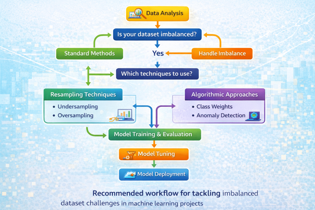
Step 1: Understand Your Data

• Calculate class distribution
• Identify imbalance ratio
• Analyze minority class characteristics
• Check for data quality issues

Step 2: Choose Appropriate Metrics

• Define business objectives
• Determine cost of different error types
• Select 2-3 relevant metrics
• Establish baseline performance

Step 3: Start Simple

• Train baseline model without adjustments
• Apply class weights as first intervention
• Evaluate improvement
• Document results

Step 4: Try Resampling

• Test random oversampling
• Compare with SMOTE
• Try combined approaches (SMOTE + Tomek)
• Select best performing method

Step 5: Experiment with Advanced Techniques

• Adjust classification threshold
• Try ensemble methods
• Consider cost-sensitive learning
• Test anomaly detection if appropriate

Step 6: Validate Thoroughly

• Use stratified k-fold cross-validation
• Check for overfitting
• Validate on separate holdout set
• Test with realistic data distributions

Step 7: Monitor in Production

• Track performance metrics over time
• Watch for distribution shift
• Retrain as needed
• Update thresholds if necessary

Common Pitfalls to Avoid

1. Resampling Before Splitting:

• Wrong: Resample entire dataset, then split into train/test
• Right: Split first, then resample only training set
• Why: Prevents data leakage and overly optimistic results

2. Ignoring Validation Strategy:

• Use stratified splits to maintain class distribution
• Ensure test set reflects real-world distribution
• Don’t resample test/validation sets

3. Overfitting to Minority Class:

• Monitor training vs. validation performance
• Use regularization techniques
• Avoid excessive oversampling

4. Using Inappropriate Metrics:

• Don’t rely solely on accuracy
• Choose metrics aligned with business objectives
• Report multiple metrics for comprehensive view

5. Not Considering Data Collection:

• If possible, collect more minority class samples
• Check for data quality issues in minority class
• Verify labels are correct

Combining Multiple Techniques

Often, combining several approaches yields best results:

Effective Combinations:

1. SMOTE + Class Weights:
   • Balance data with SMOTE
   • Fine-tune with class weights
   • Optimize threshold
2. Undersampling + Ensemble:
   • Use EasyEnsemble
   • Multiple balanced subsets
   • Combine predictions
3. SMOTE + Focal Loss + Threshold Tuning:
   • Generate synthetic samples
   • Use focal loss in neural network
   • Optimize decision threshold

Example Combined Approach:

python

from imblearn.over_sampling import SMOTE
from imblearn.pipeline import Pipeline
from sklearn.ensemble import RandomForestClassifier

# Create pipeline
pipeline = Pipeline([
    ('smote', SMOTE(random_state=42)),
    ('classifier', RandomForestClassifier(
        class_weight='balanced',
        n_estimators=100,
        random_state=42
    ))
])

# Train
pipeline.fit(X_train, y_train)

# Predict probabilities
y_proba = pipeline.predict_proba(X_test)[:, 1]

# Optimize threshold
from sklearn.metrics import f1_score
thresholds = np.arange(0.1, 0.9, 0.05)
f1_scores = [f1_score(y_test, (y_proba >= t).astype(int)) 
             for t in thresholds]
optimal_threshold = thresholds[np.argmax(f1_scores)]

# Final predictions
y_pred = (y_proba >= optimal_threshold).astype(int)

---

Case Studies and Examples

Case Study 1: Credit Card Fraud Detection

Problem:

• Dataset: 284,807 transactions
• Fraudulent transactions: 492 (0.172%)
• Extreme imbalance ratio: 577:1

Approach:

1. Started with baseline logistic regression (accuracy: 99.9%, recall: 61%)
2. Applied SMOTE to training set
3. Used class weights with XGBoost
4. Optimized threshold for F1-score
5. Implemented ensemble of models with different sampling strategies

Results:

• Baseline recall: 61%
• Final recall: 89%
• Precision maintained at 85%
• Reduced false negatives by 70%

Key Learnings:

• SMOTE worked better than random oversampling
• Ensemble approach reduced variance
• Threshold optimization crucial for production deployment
• Regular retraining needed due to evolving fraud patterns

Case Study 2: Medical Diagnosis (Rare Disease Detection)

Problem:

• Dataset: 10,000 patient records
• Positive cases: 150 (1.5%)
• High cost of false negatives (missing disease)

Approach:

1. Used cost-sensitive learning with 20:1 FN:FP cost ratio
2. Applied borderline-SMOTE for synthetic sample generation
3. Implemented ensemble of specialized models
4. Set conservative threshold (0.3) to maximize recall

Results:

• Recall increased from 72% to 94%
• Precision: 78% (acceptable given cost considerations)
• Reduced missed diagnoses by 65%
• System flagged more cases for expert review

Key Learnings:

• Domain expertise critical for setting costs
• Borderline-SMOTE generated more realistic samples
• Lower threshold appropriate given high FN cost
• Model served as screening tool, not replacement for doctors

Case Study 3: Customer Churn Prediction

Problem:

• Dataset: 50,000 customers
• Churned customers: 8,500 (17%)
• Moderate imbalance

Approach:

1. Feature engineering to capture behavioral patterns
2. Applied random undersampling to majority class
3. Used BalancedRandomForest
4. Optimized for F2-score (emphasis on recall)

Results:

• F2-score improved from 0.51 to 0.69
• Identified 82% of churners (vs. 59% baseline)
• Enabled targeted retention campaigns
• ROI: 4.2x from reduced churn

Key Learnings:

• Undersampling worked well with abundant majority class data
• Feature quality more important than sampling technique
• Business metrics (ROI) should guide metric selection
• Regular model updates needed for changing customer behavior

---

Frequently Asked Questions (FAQ)

Q1: What is considered an imbalanced dataset?

A: A dataset is generally considered imbalanced when one class has significantly fewer samples than others. While there’s no strict threshold, common guidelines are:

• Moderate imbalance: 20:80 to 40:60 ratio (1:4 to 2:3)
• Severe imbalance: Less than 10% minority class (1:10 or worse)
• Extreme imbalance: Less than 1% minority class (1:100 or worse)

The level of concern depends on your specific application, available data, and the consequences of misclassification. Even 30:70 distributions can cause problems if minority class detection is critical.

Q2: Should I always balance my dataset?

A: Not necessarily. Consider these factors:

• Severity of imbalance: Mild imbalance (40:60) may not require intervention
• Algorithm choice: Some algorithms (XGBoost, neural networks) handle imbalance well with proper configuration
• Real-world distribution: Sometimes maintaining natural distribution with adjusted thresholds is better
• Available data: With very small minority class, some techniques may not work well

Start by training a baseline model to assess whether imbalance is actually causing problems. If minority class performance is acceptable, you may not need balancing techniques.

Q3: What’s the difference between SMOTE and random oversampling?

A: The key differences are:

Random Oversampling:

• Creates exact duplicates of existing minority samples
• Fast and simple
• Risk of overfitting (model memorizes duplicates)
• Doesn’t add new information

SMOTE:

• Creates synthetic samples by interpolating between minority class neighbors
• Generates new, diverse examples
• Reduces overfitting risk
• More computationally expensive
• Can create unrealistic samples in noisy regions

Generally, SMOTE performs better for most applications, but random oversampling can work well with ensemble methods or when minority class is very small.

Q4: When should I use undersampling vs. oversampling?

A: Choose based on your situation:

Use Undersampling when:

• You have abundant majority class data (>100,000 samples)
• Training time is a concern
• You want to reduce dataset size
• Majority class contains redundant information

Use Oversampling when:

• You have limited data overall
• Preserving all information is important
• Minority class is very small
• You can afford longer training time

Use Combined Approach when:

• You have moderate amounts of data
• You want benefits of both techniques
• You’re using SMOTE-Tomek or SMOTE-ENN

Q5: How do I choose the right evaluation metric?

A: Select metrics based on your business objectives:

Use Precision when:

• False positives are very costly
• You need high confidence in positive predictions
• Example: Spam detection (false positives annoy users)

Use Recall when:

• False negatives are very costly
• You must catch most positive cases
• Example: Disease screening (missing a case is dangerous)

Use F1-Score when:

• You need balance between precision and recall
• Both error types have similar costs
• You want a single metric for comparison

Use AUC-ROC when:

• You want threshold-independent evaluation
• Classes are moderately imbalanced
• You’re comparing multiple models

Use AUC-PR when:

• Dataset is severely imbalanced
• You care more about minority class
• You want threshold-independent metric focused on positive class

Q6: Can I use both resampling and class weights together?

A: Yes, you can combine these techniques, and it often improves results. However, be careful:

Safe Combination:

• Use moderate resampling (e.g., 70% balance, not complete)
• Apply modest class weights
• Monitor for overfitting

Potential Issues:

• Over-emphasizing minority class
• Overfitting to minority patterns
• Training instability

Best Practice: Start with one technique, then incrementally add others while monitoring validation performance. Use cross-validation to ensure generalization.

Q7: How do I prevent data leakage when using resampling?

A: Follow this critical rule: Always split before resampling

Correct Workflow:

python

# 1. Split data first
X_train, X_test, y_train, y_test = train_test_split(X, y, test_size=0.2)

# 2. Apply resampling only to training set
smote = SMOTE()
X_train_resampled, y_train_resampled = smote.fit_resample(X_train, y_train)

# 3. Train model
model.fit(X_train_resampled, y_train_resampled)

# 4. Test on original test set (not resampled)
model.predict(X_test)

Never:

• Resample before splitting
• Resample validation or test sets
• Use information from test set when resampling training set

This ensures your model is evaluated on realistic, unseen data.

Q8: Which technique works best for extreme imbalance (< 1% minority class)?

A: For extreme imbalance, consider:

First Choice: Anomaly Detection

• One-Class SVM
• Isolation Forest
• Autoencoders
• Treats minority class as anomalies

Second Choice: Combination Approach

• SMOTE for synthetic sample generation
• Focal Loss in neural networks
• Ensemble methods (EasyEnsemble, BalancedRandomForest)
• Very conservative classification threshold

Third Choice: Cost-Sensitive Learning

• Assign high penalty to minority class misclassification
• Often 100:1 or higher cost ratio
• Works well with gradient boosting

Important: With extreme imbalance, collecting more minority class data (if possible) often provides better results than any algorithmic technique.

Q9: How can I handle imbalanced multi-class problems?

A: Multi-class imbalance requires adapted approaches:

Techniques:

1. One-vs-Rest with resampling: Treat each class separately against all others
2. Class weights: Set individual weights for each class
3. Multi-class SMOTE: Generate synthetic samples for all minority classes
4. Hierarchical classification: Group similar rare classes together

Implementation Example:

python

from imblearn.over_sampling import SMOTE

# SMOTE handles multi-class automatically
smote = SMOTE(sampling_strategy='not majority')  # Oversample all minority classes
X_resampled, y_resampled = smote.fit_resample(X_train, y_train)

# Or specify custom strategy
sampling_strategy = {0: 1000, 1: 1000, 2: 500}  # Target samples for each class
smote = SMOTE(sampling_strategy=sampling_strategy)

Best Practice: Focus on the rarest classes first, then progressively address others.

Q10: How often should I retrain models on imbalanced data?

A: Retraining frequency depends on:

Monitor These Signals:

• Performance degradation on validation set
• Distribution shift in incoming data
• Changes in minority class patterns (e.g., new fraud techniques)
• Seasonal variations in your domain

General Guidelines:

• Static domains: Retrain quarterly or when performance drops >5%
• Dynamic domains (fraud, spam): Retrain monthly or even weekly
• Stable domains (medical): Retrain annually or with new research

Best Practice:

• Implement automated performance monitoring
• Set performance thresholds that trigger retraining
• Keep recent historical data for continuous improvement
• A/B test new models before full deployment

---

Conclusion

Dealing with imbalanced datasets is a fundamental challenge in machine learning that requires thoughtful strategy and appropriate techniques. Throughout this guide, we’ve explored comprehensive solutions ranging from basic resampling methods to advanced algorithmic approaches.

Key Takeaways:

1. Understand Your Problem: The severity of imbalance, domain requirements, and business costs should guide your approach
2. Choose Appropriate Metrics: Accuracy is misleading—use precision, recall, F1-score, or AUC-PR instead
3. Start Simple: Begin with class weights or basic resampling before trying complex methods
4. Avoid Data Leakage: Always split data before resampling, and never resample test sets
5. Combine Techniques: Hybrid approaches (SMOTE + class weights, ensemble + resampling) often work best
6. Validate Thoroughly: Use stratified cross-validation and monitor for overfitting
7. Monitor Production: Track performance metrics and retrain as needed

Moving Forward:

The field continues to evolve with new techniques emerging regularly. Stay current by:

• Experimenting with different approaches on your specific data
• Monitoring latest research in imbalanced learning
• Participating in Kaggle competitions with imbalanced datasets
• Sharing experiences with the data science community

Remember, there’s no one-size-fits-all solution. The best approach depends on your specific dataset, domain, and business requirements. Start with fundamentals, experiment systematically, and always validate thoroughly before deploying to production.

By mastering these techniques, you’ll be well-equipped to build robust, reliable models that perform effectively even with severely imbalanced datasets—whether you’re detecting fraud, diagnosing diseases, predicting churn, or solving any other classification challenge where minority class detection matters.

Additional Resources:

• Imbalanced-learn library documentation
• Scikit-learn user guide on imbalanced datasets
• Research papers on novel resampling techniques
• Domain-specific best practices for your industry