Introduction of Feature Engineering Techniques
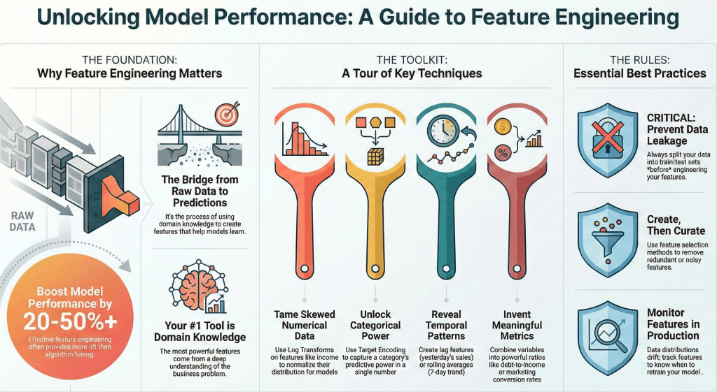
In the world of machine learning, there’s a well-known saying: “garbage in, garbage out.” While sophisticated algorithms often steal the spotlight, the true differentiator between mediocre and exceptional models lies in feature engineering. According to industry research, feature engineering can improve model performance by 20-50% or more, often outperforming the gains from algorithm selection or hyperparameter tuning.
Feature engineering is both an art and a science—it requires domain expertise, creativity, and a deep understanding of your data. This comprehensive guide explores proven feature engineering techniques that consistently deliver measurable improvements in model performance across various machine learning applications.
Whether you’re working on classification, regression, or time series forecasting, the techniques covered in this article will help you extract maximum value from your data and build models that truly perform in production environments.
Understanding Feature Engineering
Feature engineering is the process of using domain knowledge to create, transform, and select variables (features) that make machine learning algorithms work more effectively. It’s the bridge between raw data and actionable predictions.
Why Feature Engineering Matters:
Good features make it easier for algorithms to learn patterns. They can reduce model complexity, improve interpretability, decrease training time, and significantly boost predictive accuracy. A well-engineered feature can capture complex relationships that would require deep neural networks to learn from raw data.
The Feature Engineering Mindset:
Successful feature engineering requires understanding your business problem, exploring data distributions and relationships, thinking creatively about what information might be predictive, and iterating based on model performance feedback.
Before diving into techniques, it’s crucial to have clean, well-understood data. Perform exploratory data analysis to understand distributions, identify outliers, and recognize missing value patterns. This foundation informs your feature engineering decisions.
Core Feature Engineering Techniques
Numerical Transformations
Numerical features often benefit from transformations that make their distributions more suitable for machine learning algorithms.
Log Transformations: When dealing with right-skewed data (like income, prices, or counts), log transformations can normalize distributions and reduce the impact of outliers. For a feature X, apply log(X + 1) or log(X + c) where c is a small constant to handle zero values.

This technique is particularly valuable for features spanning multiple orders of magnitude. For example, transforming website traffic data (ranging from 10 to 100,000 visitors) using log transformation helps models treat relative changes (10 to 100 vs. 1,000 to 10,000) more appropriately.
Power Transformations: Box-Cox and Yeo-Johnson transformations automatically find the optimal power transformation for your data. These techniques are more sophisticated than simple log transforms and can handle both positive and negative values (Yeo-Johnson) or strictly positive values (Box-Cox).
Binning and Discretization: Converting continuous variables into categorical bins can capture non-linear relationships. For instance, age groups (18-25, 26-35, 36-50, 51+) might be more predictive than raw age in customer segmentation. However, use binning judiciously—you lose granularity and information.
Quantile-based binning ensures equal distribution across bins, while custom bins based on domain knowledge often yield better results. For credit scoring, you might bin income based on regulatory thresholds or lending policy brackets.
Categorical Encoding
Categorical variables require special treatment since most machine learning algorithms work with numerical inputs.

One-Hot Encoding: The most common approach creates binary columns for each category. For a “color” feature with values [red, blue, green], you create three binary columns: is_red, is_blue, is_green. This works well for low-cardinality features (fewer than 10-15 unique values).
However, one-hot encoding can create dimensionality problems with high-cardinality features. A zip code feature with 1,000 unique values creates 1,000 new columns, leading to sparse matrices and increased computational costs.
Target Encoding: Replace categories with statistics derived from the target variable. For example, in a binary classification problem, replace each category with the mean target value for that category. This captures the predictive power of categories in a single numerical feature.
Target encoding is powerful but prone to overfitting, especially with small sample sizes. Always use cross-validation techniques or smoothing methods to prevent data leakage. Add the overall mean weighted by category frequency to smooth target encoding and prevent overfitting on rare categories.
Frequency Encoding: Replace categories with their frequency count or percentage in the dataset. This simple technique works surprisingly well when the frequency itself is predictive. For instance, in fraud detection, rare user agents or IP addresses might indicate suspicious activity.
Embedding Encoding: For high-cardinality categorical features, learned embeddings (like those used in neural networks) can compress categories into dense vectors that capture semantic relationships. This technique is particularly powerful when you have enough data to train meaningful embeddings.
Feature Scaling and Normalization
Many algorithms (SVM, neural networks, k-nearest neighbors) are sensitive to feature scales. Proper scaling ensures all features contribute appropriately to model predictions.

Min-Max Scaling: Transforms features to a fixed range, typically [0, 1]. Formula: (X – X_min) / (X_max – X_min). This preserves the original distribution shape but is sensitive to outliers.
Use min-max scaling when you need bounded features or when working with algorithms that assume input in specific ranges (like neural networks with sigmoid activation).
Standard Scaling (Z-score Normalization): Transforms features to have mean zero and standard deviation one. Formula: (X – mean) / std_dev. This is less sensitive to outliers than min-max scaling and is preferred for many algorithms.
Standard scaling assumes your data follows a roughly Gaussian distribution. It’s the go-to choice for linear models, support vector machines, and neural networks.
Robust Scaling: Uses median and interquartile range instead of mean and standard deviation, making it robust to outliers. Formula: (X – median) / IQR. Choose this when your data contains significant outliers that you want to preserve as information rather than treat as noise.
Important: Always fit scalers on training data only, then apply the same transformation to validation and test sets to prevent data leakage.
Feature Creation and Interaction
Creating new features by combining existing ones often captures relationships that improve model performance.
Polynomial Features: Create interaction terms and polynomial terms from existing features. For features X and Y, generate X², Y², and X*Y. This allows linear models to capture non-linear relationships.
However, polynomial features explode dimensionally. With 10 features, degree-2 polynomials create 65 features. Use feature selection techniques to identify the most valuable polynomial terms.
Ratio Features: Creating ratios between related features often captures meaningful business metrics. Examples include debt-to-income ratio in credit scoring, conversion rate (conversions / visits) in marketing analytics, and revenue per employee in business analytics.
Ratio features are particularly powerful when they encode domain knowledge about what matters in your problem space. Think about what key performance indicators exist in your domain and create features that represent them.
Arithmetic Combinations: Simple addition, subtraction, multiplication, and division of related features can reveal patterns. For e-commerce, you might create total_spend = price * quantity, or discount_percentage = (original_price – sale_price) / original_price.
Distance and Similarity Features: Calculate distances between data points and reference points. For geographic data, distance to city center, nearest store, or competitor location can be highly predictive. For customer analytics, similarity to high-value customer segments provides useful signal.
Time-Based Features
Temporal data contains rich information that requires specialized feature engineering.

Date-Time Decomposition: Extract components from timestamps: year, month, day, day of week, hour, minute, quarter, week of year. Each component can capture different seasonal patterns.
Day of week is particularly powerful for retail and web traffic prediction. Hour of day matters for energy consumption forecasting. Month and quarter capture annual seasonality.
Cyclical Encoding: Time features like hour (0-23) and month (1-12) are cyclical—December is close to January, and 11 PM is close to midnight. Standard encoding treats them as linear, which is incorrect.
Encode cyclical features using sine and cosine transformations. For hour: hour_sin = sin(2 * π * hour / 24) and hour_cos = cos(2 * π * hour / 24). This preserves the circular nature of temporal features.
Lag Features: Create features from previous time steps. For time series forecasting, yesterday’s value, last week’s value, and same day last year are often highly predictive. Lag features capture temporal dependencies and autocorrelation.
Experiment with multiple lag periods based on your domain. Retail sales might need daily, weekly, and yearly lags. Stock prices might need hourly, daily, and weekly lags.
Rolling Statistics: Calculate moving averages, rolling standard deviations, and other rolling window statistics. These features smooth out noise and capture trends. A 7-day moving average reveals weekly trends, while a 30-day rolling standard deviation captures volatility.
Time Since Events: Calculate time elapsed since important events: days since last purchase, time since account creation, hours since last login. These features capture recency effects that are powerful predictors in many domains.
Text Feature Engineering
Text data requires transformation into numerical representations that algorithms can process.
TF-IDF (Term Frequency-Inverse Document Frequency): Weights words by their frequency in a document relative to their frequency across all documents. This highlights distinctive words while downweighting common terms like “the” and “is.”

TF-IDF creates sparse but interpretable features. It works well for moderate-sized text datasets and provides a strong baseline for text classification tasks.
Word Embeddings: Pre-trained embeddings like Word2Vec, GloVe, or BERT capture semantic relationships between words. Words with similar meanings have similar vector representations, enabling models to generalize across synonyms.
Average or max-pool word embeddings across documents to create document-level features. For longer texts, sentence embeddings from models like Sentence-BERT provide better representations.
N-grams: Capture word sequences by creating features from consecutive word combinations. Bigrams (2-word sequences) and trigrams (3-word sequences) preserve some word order information that single-word features miss.
The phrase “not good” has very different meaning than “good,” which n-grams can capture while individual word features cannot.
Text Statistics: Extract numerical features from text: document length, average word length, sentence count, punctuation frequency, capitalization patterns, and presence of special characters.
For product reviews, length and punctuation patterns help predict review rating. For email classification, presence of certain characters or URL patterns helps identify spam.
Domain-Specific Text Features: Create features based on domain knowledge: presence of specific keywords, sentiment scores, readability metrics, named entity counts, and industry-specific terminology frequency.
Advanced Feature Engineering Methods
Domain-Specific Features
The most powerful features often come from deep domain expertise.
E-commerce and Retail: Create features like customer lifetime value metrics, purchase frequency buckets, average basket size, time between purchases, product category preferences, price sensitivity indicators (response to discounts), and seasonal buying patterns.

Finance and Credit Scoring: Engineer features such as debt-to-income ratios, payment history indicators, credit utilization rates, account age metrics, recent inquiry counts, and stability indicators (job tenure, residence duration).
Healthcare and Medical: Develop features like risk scores based on condition combinations, medication interaction flags, vital sign trends over time, seasonal health patterns, and demographic risk factors.
Marketing and Customer Analytics: Build features including engagement scores, channel preference indicators, campaign response history, customer journey stage, and cohort-based metrics.
Domain expertise helps you identify which raw data elements contain predictive signal and how to combine them meaningfully. Spend time with subject matter experts to understand what drives outcomes in your problem space.
Automated Feature Engineering
While manual feature engineering remains valuable, automated approaches can accelerate the process and discover non-obvious patterns.
Featuretools: This Python library performs automated feature engineering using deep feature synthesis. It automatically creates features by stacking operations and aggregations across related tables.
Featuretools excels at relational datasets where entities are connected. It can automatically create time-aware aggregations, handle temporal relationships, and generate hundreds or thousands of features.
However, automated feature engineering requires validation. Not all generated features improve performance—many may be redundant or noisy. Always pair automated generation with feature selection.
Polynomial Feature Generation: While simple, automatically generating polynomial terms and interactions up to a specified degree can reveal non-linear patterns. Scikit-learn’s PolynomialFeatures makes this straightforward.
Balance the degree of polynomial features with model complexity. Higher degrees capture more complex patterns but dramatically increase dimensionality and overfitting risk.
Genetic Programming: Techniques like TPOT (Tree-based Pipeline Optimization Tool) use genetic algorithms to evolve feature engineering operations alongside model selection and hyperparameters.
These meta-learning approaches can discover creative feature combinations but require significant computational resources and careful validation to avoid overfitting to your validation set.
Feature Selection Techniques
Creating features is only half the battle—selecting the right subset is equally important.
Filter Methods: Evaluate features independently of the model using statistical tests. Correlation analysis identifies features strongly related to the target. Mutual information measures dependence between variables, capturing non-linear relationships that correlation misses.
Chi-square tests work well for categorical features in classification problems. ANOVA F-tests suit numerical features.
Filter methods are fast and model-agnostic but don’t account for feature interactions or redundancy.
Wrapper Methods: Evaluate feature subsets based on model performance. Recursive Feature Elimination (RFE) iteratively removes the least important features based on model coefficients or feature importance scores.
Forward selection starts with no features and adds them one by one. Backward elimination starts with all features and removes them iteratively. These methods are computationally expensive but account for feature interactions.
Embedded Methods: Feature selection occurs during model training. L1 regularization (Lasso) automatically performs feature selection by shrinking some coefficients to zero. Tree-based models provide feature importance scores based on how often features are used for splitting and the reduction in impurity they achieve.
Embedded methods balance computational efficiency with considering feature interactions. They’re particularly effective when your final model will use the same algorithm family.
Practical Feature Selection Strategy: Start with domain knowledge to remove obviously irrelevant features. Apply correlation analysis to remove highly correlated redundant features. Use model-based importance scores (from random forests or gradient boosting) to identify top candidates. Perform ablation studies—systematically remove features and measure performance impact. Validate on held-out test sets to ensure selected features generalize.
Real-World Impact: Performance Metrics
Feature engineering’s impact on model performance is substantial and measurable across diverse applications.

Kaggle Competition Insights: Analysis of winning Kaggle solutions reveals that top performers typically spend 60-80% of their time on feature engineering compared to 20-40% on model selection and tuning. Winners often create 50-500 engineered features from just 10-50 raw features.
In the Taxi Trip Duration competition, winners achieved dramatic improvements through feature engineering: distance features calculated from coordinates, time-based features (rush hour indicators, day of week), weather data integration, and traffic pattern features.
Business Impact Examples:
In credit risk modeling, proper feature engineering can reduce default prediction error by 25-40% compared to using raw features. Key improvements come from ratio features (debt-to-income), time-based features (payment history patterns), and aggregation features (average balance, maximum utilization).
For e-commerce recommendation systems, engagement features (click-through patterns, time-on-page distributions) combined with collaborative filtering features improve conversion predictions by 30-50%.
Churn prediction models benefit substantially from behavioral change features. Detecting decreasing engagement trends through rolling window statistics often provides more signal than snapshot features, improving AUC from 0.75 to 0.85+.
Computational Efficiency: Well-engineered features can reduce model complexity. Capturing key patterns in features allows simpler models to achieve the same or better performance than complex models on raw data. This means faster training, easier deployment, reduced infrastructure costs, and improved model interpretability.
A logistics company reduced model training time from 6 hours to 45 minutes by engineering features that captured complex temporal patterns, allowing them to use gradient boosting instead of deep learning while maintaining prediction accuracy.
Best Practices and Common Pitfalls
Data Leakage Prevention: The most critical concern in feature engineering is preventing data leakage—when information from the target or future leaks into features.
Common leakage sources include using future information in time series problems, calculating statistics including the target row, applying transformations before train-test split, and using test set information to select or engineer features.
Always split data before feature engineering or fit transformations. Use cross-validation properly—fit scalers and encoders on each fold’s training set only. Be especially careful with target encoding and time series features.
Handle Missing Values Thoughtfully: Missing values often contain information—the fact that data is missing might be predictive. Create binary indicator features for missingness before imputation.
Choose imputation strategies based on why data is missing: mean/median imputation for random missingness, forward fill for time series, model-based imputation (like KNN or iterative imputer) when missingness has patterns, and domain-specific imputation based on business logic.
Feature Engineering Pipeline: Treat feature engineering as code—use version control, write reusable transformation functions, document feature definitions and rationale, and create automated testing to catch engineering errors.
Structure your pipeline to ensure reproducibility: separate feature engineering code from model training, make transformation parameters explicit and configurable, and log feature engineering decisions and their performance impact.
Avoid Over-Engineering: More features don’t always mean better models. Too many features can lead to overfitting, increase computational costs, reduce model interpretability, and make deployment more complex.
Focus on features that add unique information. Remove redundant features through correlation analysis or feature selection. Start with simple features before creating complex ones. Validate that each feature genuinely improves out-of-sample performance.
Domain Knowledge Integration: The best features come from understanding your problem domain. Work closely with subject matter experts, understand the business process generating your data, research similar problems and successful feature engineering approaches, and think about causal relationships, not just correlations.
Ask “why would this predict the outcome?” when creating features. Features based on sound reasoning are more likely to generalize.
Iteration and Experimentation: Feature engineering is inherently experimental. Track all experiments systematically, measure performance impact of each feature set, use proper validation methodology, and iterate based on both quantitative metrics and qualitative insights.
Modern experiment tracking tools (MLflow, Weights & Biases) help manage feature engineering experiments alongside model experiments.
Implementation Strategies
Start Simple: Begin with basic transformations and encodings. Establish a solid baseline before adding complexity. Simple features often provide 80% of the value with 20% of the effort.

Iterative Approach: Add features in groups and measure incremental impact. This helps identify which types of features are most valuable for your specific problem and prevents drowning in complexity.
Cross-Validation is Essential: Always validate feature engineering decisions using proper cross-validation. Single train-test splits can be misleading, especially with small datasets. K-fold cross-validation provides more robust performance estimates.
For time series, use time-based splitting that respects temporal order—train on past data, predict future data.
Feature Engineering Checklist:
Before production deployment, verify: all features can be computed at prediction time, no data leakage exists in feature construction, missing value handling is robust and documented, feature distributions are similar in training and deployment, computational requirements are acceptable for production latency requirements, and all features are clearly documented with definitions and rationale.
Tools and Libraries:
Python offers excellent feature engineering tools: pandas for data manipulation and basic transformations, scikit-learn for preprocessing, encoding, and scaling, featuretools for automated feature engineering, category_encoders for advanced encoding methods, and tsfresh for time series feature extraction.
For production deployment, consider tools like feature stores (Feast, Tecton) that manage feature computation, storage, and serving across training and production.
Monitoring in Production: Feature distributions can drift over time. Monitor feature statistics in production, set up alerts for unusual feature values or distributions, track feature importance over time, and regularly retrain and re-engineer features as patterns change.
Conclusion
Feature engineering remains one of the most impactful activities in machine learning. While automated machine learning and deep learning have made some feature engineering automatic, domain-driven feature engineering continues to deliver superior results in most applied machine learning problems.
The techniques covered in this article—numerical transformations, categorical encoding, feature scaling, feature creation, time-based features, text features, domain-specific engineering, automated approaches, and feature selection—form a comprehensive toolkit for improving model performance.
Remember that feature engineering is both art and science. It requires creativity, domain knowledge, technical skill, and rigorous validation. The best features often come from deep understanding of your problem domain combined with systematic experimentation.
As you develop your feature engineering skills, focus on understanding why features work, not just that they work. This understanding helps you transfer techniques across problems and create novel features for new challenges.
Start with the fundamentals, experiment systematically, validate rigorously, and always keep the end goal in mind—building models that perform reliably in production environments.
The time invested in thoughtful feature engineering pays dividends throughout the entire machine learning lifecycle, from initial model development through production deployment and maintenance.
Key Takeaways:
Feature engineering can improve model performance by 20-50% or more. Good features reduce model complexity and improve interpretability. Domain knowledge is your most powerful feature engineering tool. Prevent data leakage through careful validation methodology. Iterate systematically and measure incremental impact. Balance feature creation with feature selection. Monitor features in production as data distributions drift.
Master these techniques, and you’ll build machine learning models that truly perform when it matters most.