Data transformation is the cornerstone of successful machine learning and data analysis projects. Whether you’re building predictive models, conducting statistical analysis, or preparing data for visualization, understanding data transformation methods like normalization, standardization, and encoding is absolutely essential for achieving optimal results.

In this comprehensive guide, we’ll explore the three fundamental data transformation techniques that every data scientist, analyst, and machine learning engineer must master. You’ll learn when to use each method, how to implement them effectively, and understand their impact on your machine learning models and data preprocessing pipelines.
🎯 What You’ll Learn:
- The difference between normalization and standardization
- When to use each data transformation method
- Practical implementation examples for data preprocessing
- Encoding techniques for categorical variables
- Best practices for feature scaling in machine learning
Understanding Data Transformation: The Foundation of Data Preprocessing

Data transformation refers to the process of converting data from one format or structure into another to make it suitable for analysis or machine learning algorithms. In the context of data preprocessing, transformation methods are crucial for ensuring that different features are on comparable scales and that categorical variables are properly represented for computational processing.
Raw datasets often contain features with vastly different ranges, units, and distributions. For instance, a dataset might include age (ranging from 0-100), salary (ranging from 20,000-200,000), and credit score (ranging from 300-850). Without proper data transformation and feature scaling, machine learning algorithms can become biased toward features with larger magnitudes, leading to suboptimal model performance.
💡 Key Insight: Most machine learning algorithms, particularly distance-based algorithms like K-Nearest Neighbors (KNN), Support Vector Machines (SVM), and neural networks, are sensitive to the scale of input features. Proper data transformation ensures that all features contribute equally to the model’s learning process.
Why Data Transformation is Critical for Machine Learning
The importance of data transformation in machine learning cannot be overstated. Here are the primary reasons why feature scaling and data normalization are essential:
Faster Convergence: Algorithms that use gradient descent, such as neural networks and logistic regression, converge much faster when features are on similar scales. Without proper standardization or normalization, the optimization process can take significantly longer or even fail to converge.
Improved Model Performance: Many algorithms calculate distances between data points. When features have different scales, those with larger ranges dominate the distance calculations, effectively reducing the influence of other features. Data scaling techniques ensure all features have equal weight.
Enhanced Interpretability: When features are on comparable scales, model coefficients and feature importance scores become more interpretable, allowing for better understanding of which variables drive predictions.
Normalization: Scaling Data to a Fixed Range

Normalization, also known as min-max scaling or min-max normalization, is a data transformation technique that rescales features to a fixed range, typically between 0 and 1. This feature scaling method preserves the original distribution of the data while ensuring all values fall within the specified range.
The Min-Max Normalization Formula
The mathematical formula for min-max normalization is straightforward and elegant:
X_normalized = (X - X_min) / (X_max - X_min)
Where:
- X is the original value
- X_min is the minimum value in the feature
- X_max is the maximum value in the feature -
X_normalized is the normalized value (between 0 and 1)
When to Use Normalization
Normalization techniques are particularly effective in the following scenarios:
Neural Networks and Deep Learning: Neural networks work best when input features are within a bounded range. Data normalization to the [0,1] range helps activation functions like sigmoid and tanh operate in their most sensitive regions, improving gradient flow during backpropagation.
Image Processing: In computer vision applications, pixel values are typically normalized to the [0,1] range, making min-max normalization the natural choice for image data preprocessing.
Bounded Algorithms: Algorithms that assume features are within a specific range, such as certain distance-based methods or algorithms that use bounded activation functions, benefit significantly from normalization.
Known Range Requirements: When your model or business logic requires features to be within a specific range, min-max scaling provides precise control over the output bounds.
Practical Normalization Example
Let’s walk through a concrete example of data normalization in practice:
# Python Example: Min-Max Normalization
import numpy as np from sklearn.preprocessing
import MinMaxScaler
# Original data: House prices in thousands
house_prices = np.array([[150], [200], [250], [300], [500]])
# Create and apply Min-Max Scaler
scaler = MinMaxScaler()
normalized_prices = scaler.fit_transform(house_prices)
print("Original Prices:", house_prices.flatten())
# Output: [150, 200, 250, 300, 500]
print("Normalized Prices:", normalized_prices.flatten())
# Output: [0.0, 0.143, 0.286, 0.429, 1.0]
# Manual calculation for verification:
# For price 200: (200 - 150) / (500 - 150) = 50/350 = 0.143
⚠️ Important Consideration: Normalization is sensitive to outliers because it uses the minimum and maximum values of the dataset. A single extreme value can compress the rest of your data into a small range, reducing the effectiveness of the normalization. Consider outlier detection and treatment before applying min-max normalization.
Standardization: Centering Data Around the Mean

Standardization, also referred to as z-score normalization or z-score standardization, is a data scaling technique that transforms features to have a mean of zero and a standard deviation of one. Unlike normalization, standardization doesn’t bound values to a specific range but instead centers the data around zero.
The Standardization Formula
The z-score standardization formula is based on statistical measures:
Z = (X - μ) / σ
Where:
- X is the original value
- μ (mu) is the mean of the feature
- σ (sigma) is the standard deviation of the feature
- Z is the standardized value (z-score)
When to Use Standardization
Standardization methods are preferred in these situations:
Gaussian Distribution Assumptions: Many machine learning algorithms, including linear regression, logistic regression, and linear discriminant analysis, assume that features follow a Gaussian (normal) distribution. Z-score standardization helps meet this assumption by centering the data.
Principal Component Analysis (PCA): PCA and feature scaling go hand-in-hand. Since PCA is sensitive to the variance of features, standardization ensures that all features contribute proportionally to the principal components.
Distance-Based Algorithms: Algorithms like K-Means clustering, KNN, and SVM that rely on distance metrics perform better with standardized features, as it prevents features with larger scales from dominating distance calculations.
Presence of Outliers: Unlike normalization, standardization is more robust to outliers because it uses mean and standard deviation rather than minimum and maximum values, making it a better choice for data preprocessing with outliers.
Practical Standardization Example
# Python Example: Z-Score Standardization
import numpy as np from sklearn.preprocessing
import StandardScaler
# Original data: Test scores
test_scores = np.array([[65], [70], [75], [80], [85], [90], [95]])
# Create and apply Standard Scaler
scaler = StandardScaler()
standardized_scores = scaler.fit_transform(test_scores)
print("Original Scores:", test_scores.flatten())
# Output: [65, 70, 75, 80, 85, 90, 95]
print("Mean:", scaler.mean_[0])
# Output: 80.0 print("Standard Deviation:", np.sqrt(scaler.var_[0]))
# Output: 10.0 print("Standardized Scores:", standardized_scores.flatten().round(2))
# Output: [-1.5, -1.0, -0.5, 0.0, 0.5, 1.0, 1.5]
# Manual calculation for score 65: # (65 - 80) / 10 = -1.5
Normalization vs Standardization: Making the Right Choice
Understanding the distinction between normalization and standardization is crucial for effective data preprocessing. Here’s a comprehensive comparison to guide your decision:
| Aspect | Normalization (Min-Max) | Standardization (Z-Score) |
|---|---|---|
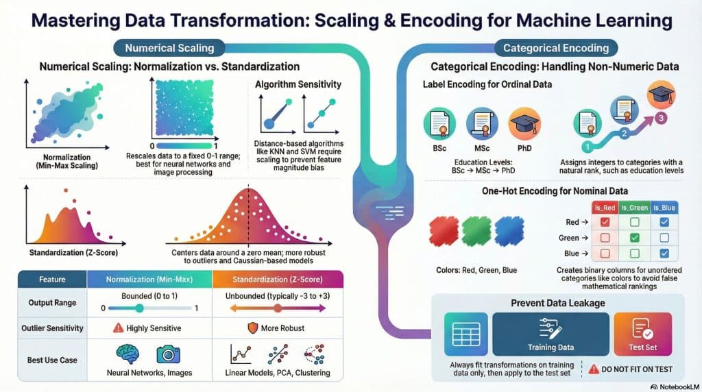
| Output Range | Bounded (typically 0 to 1) | Unbounded (typically -3 to +3) |
| Outlier Sensitivity | Highly sensitive | More robust |
| Distribution Assumption | No assumption | Works best with Gaussian |
| Best Use Cases | Neural networks, bounded ranges | Linear models, PCA, clustering |
| Maintains Distribution Shape | Yes | Yes |
| Formula Base | Min and Max values | Mean and Standard Deviation |
🎯 Quick Decision Guide: Use normalization when you need bounded values (0-1) and your data doesn’t have significant outliers. Use standardization when you’re working with algorithms that assume normal distribution, when dealing with outliers, or when the absolute range isn’t important but the relative distribution is.
Encoding: Transforming Categorical Data for Machine Learning

Categorical encoding is the process of converting categorical variables (non-numeric data) into numeric format that machine learning algorithms can process. Since most ML algorithms require numeric input, encoding categorical data is an essential step in data preprocessing pipelines.
Types of Categorical Variables
Before diving into encoding methods, it’s important to understand the two main types of categorical variables:
Nominal Categories: These are categories without any inherent order or ranking. Examples include color (red, blue, green), country names, or product categories. For nominal categorical variables, the order in which they appear has no meaning.
Ordinal Categories: These categories have a meaningful order or ranking. Examples include education level (high school, bachelor’s, master’s, PhD), rating scales (poor, fair, good, excellent), or t-shirt sizes (S, M, L, XL). The order matters for ordinal categorical encoding.
Label Encoding: Simple Numeric Assignment
Label encoding assigns a unique integer to each category. This is the simplest form of categorical variable encoding and works well for ordinal categories.
# Python Example: Label Encoding
from sklearn.preprocessing import LabelEncoder
# Original data: Education levels (ordinal)
education = ['High School', 'Bachelor', 'Master', 'PhD', 'Bachelor', 'High School', 'Master']
# Apply Label Encoding
encoder = LabelEncoder()
encoded_education = encoder.fit_transform(education)
print("Original:", education)
print("Encoded:", encoded_education)
# Output: [1, 0, 2, 3, 0, 1, 2]
# Classes mapping print("Classes:", encoder.classes_)
# Output: ['Bachelor' 'High School' 'Master' 'PhD']
⚠️ Label Encoding Caution: While label encoding is efficient, it can introduce unintended ordinal relationships in nominal data. If you encode colors as Red=0, Green=1, Blue=2, the algorithm might incorrectly interpret that Blue > Green > Red, which is meaningless. For nominal categories, use one-hot encoding instead.
One-Hot Encoding: Creating Binary Columns
One-hot encoding, also called dummy variable encoding, creates binary columns for each category. This is the preferred method for encoding nominal categorical variables as it doesn’t impose any ordinal relationship.
Advanced Encoding Techniques for Data Scientists
Beyond basic label and one-hot encoding, several advanced categorical encoding techniques exist for specific scenarios:
Target Encoding (Mean Encoding): This powerful technique replaces each category with the mean of the target variable for that category. It’s particularly useful for high-cardinality categorical features (features with many unique categories) but requires careful implementation to avoid data leakage.
Frequency Encoding: Categories are encoded based on their frequency in the dataset. More common categories get higher values. This method works well when the frequency of a category contains predictive information.
Binary Encoding: A hybrid approach that first converts categories to integers (like label encoding) and then converts those integers to binary code. This creates fewer columns than one-hot encoding while avoiding the ordinal assumptions of label encoding, making it ideal for high-cardinality features.
# Python Example: Target Encoding (with precautions against leakage)
import pandas as pd
from sklearn.model_selection import KFold
import numpy as np
# Sample data
data = pd.DataFrame({ 'City': ['NYC', 'LA', 'Chicago', 'NYC', 'LA', 'Chicago', 'NYC'], 'Sales': [100, 150, 120, 110, 160, 130, 105] })
# Target encoding with cross-validation to prevent leakage
def target_encode_cv(df, feature, target, n_folds=5):
kf = KFold(n_splits=n_folds, shuffle=True, random_state=42)
encoded_feature = np.zeros(len(df)) for train_idx, val_idx in kf.split(df):
# Calculate mean target for each category using training fold
target_means = df.iloc[train_idx].groupby(feature)[target].mean()
# Apply to validation fold
encoded_feature[val_idx] = df.iloc[val_idx][feature].map(target_means)
return encoded_feature
# Apply target encoding
data['City_Encoded'] = target_encode_cv(data, 'City', 'Sales')
print(data)
Best Practices for Data Transformation in Machine Learning
Implementing data transformation best practices ensures your machine learning pipeline is robust, reproducible, and delivers optimal performance. Here are essential guidelines for effective data preprocessing:
1. Always Use Training Data Statistics
A critical rule in machine learning data preprocessing: always fit your transformation (normalization, standardization, or encoding) on the training data only, then apply those same transformations to validation and test sets. This prevents data leakage and ensures your model evaluation is realistic.
# CORRECT approach: Fit on training data, transform all sets
from sklearn.preprocessing import StandardScaler
from sklearn.model_selection import train_test_split
# Split data first
X_train, X_test, y_train, y_test = train_test_split(X, y, test_size=0.2)
# Fit scaler on training data only
scaler = StandardScaler() scaler.fit(X_train)
# Transform both sets using training statistics
X_train_scaled = scaler.transform(X_train)
X_test_scaled = scaler.transform(X_test)
# INCORRECT: Fitting on entire dataset
# scaler.fit(X)
# This causes data leakage!
2. Handle Outliers Before Transformation
Especially for normalization, outliers can severely distort your scaled data. Always perform outlier detection and treatment as part of your data preprocessing workflow before applying transformation methods.
3. Choose Encoding Based on Cardinality
For categorical features with low cardinality (few unique values), one-hot encoding works well. For high cardinality features (many unique values), consider target encoding, frequency encoding, or binary encoding to avoid creating too many columns.
4. Document Your Transformation Pipeline
Maintain clear documentation of which data transformation methods you applied to each feature. This ensures reproducibility and makes it easier to apply the same transformations to new data during model deployment.
❓ Frequently Asked Questions
Everything you need to know about data transformation methods
📝 Data Transformation Knowledge Quiz
Test your understanding of normalization, standardization, and encoding concepts. Answer all 7 questions and see how well you’ve mastered these essential data preprocessing techniques!
Conclusion: Mastering Data Transformation for Better Machine Learning
Data transformation methods — including normalization, standardization, and encoding — form the foundation of effective data preprocessing and successful machine learning projects. Understanding when and how to apply these techniques can dramatically improve your model’s performance, training speed, and generalization ability.
Remember these key takeaways as you implement data transformation in your ML pipeline:
Choose the right scaling method: Use normalization (min-max scaling) when you need bounded values and your data doesn’t have significant outliers. Opt for standardization (z-score) when working with algorithms that assume normal distribution, dealing with outliers, or when unbounded ranges are acceptable.
Select appropriate encoding: For categorical variables, use one-hot encoding for nominal features with low cardinality, label encoding for ordinal features, and advanced techniques like target encoding or binary encoding for high-cardinality features.
Prevent data leakage: Always fit your transformations on training data only and apply the same transformations to test and validation sets. This ensures realistic model evaluation and prevents overoptimistic performance estimates.
Consider algorithm requirements: Different algorithms have different sensitivities to feature scaling. Distance-based algorithms (KNN, SVM, neural networks) benefit greatly from scaling, while tree-based methods (Random Forest, XGBoost) are generally scale-invariant but still require proper categorical encoding.
By mastering these data transformation techniques, you’ll be well-equipped to handle diverse datasets, optimize your machine learning workflows, and build more accurate, robust predictive models. Whether you’re working on computer vision, natural language processing, or traditional tabular data, proper data transformation is your pathway to superior model performance.
🚀 Next Steps: Practice implementing these data transformation methods on real datasets. Start with scikit-learn’s preprocessing module, experiment with different techniques, and monitor their impact on your model’s performance metrics. Remember that the best transformation method often depends on your specific data characteristics and problem domain!