Understanding the Data Science Lifecycle: From Problem to Production

Introduction: The Journey from Raw Data to Business Value

In today’s data-driven world, organizations are sitting on mountains of information, yet many struggle to transform this raw data into actionable insights. The data science lifecycle provides a structured framework that guides data scientists, machine learning engineers, and business stakeholders through the complex journey from identifying a business problem to deploying production-ready solutions that deliver measurable value.

Understanding the end-to-end data science process is crucial for anyone involved in analytics, artificial intelligence, or business intelligence initiatives. Whether you’re building predictive models, recommendation systems, or automated decision-making tools, following a systematic approach ensures that your projects stay on track, meet business objectives, and scale effectively in production environments.

This comprehensive guide will walk you through each stage of the data science lifecycle, providing real-world examples, practical tips, and industry best practices that you can apply immediately to your own projects. By the end of this article, you’ll have a clear roadmap for navigating the entire journey from problem definition to production deployment.

Stage 1: Business Understanding and Problem Definition

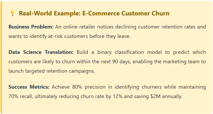
The foundation of every successful data science project is a crystal-clear understanding of the business problem you’re trying to solve. This stage involves close collaboration with stakeholders to translate business challenges into well-defined data science problems with measurable objectives.

Key Activities in This Stage:

• Stakeholder Interviews: Meet with business leaders, domain experts, and end-users to understand pain points, current processes, and desired outcomes.
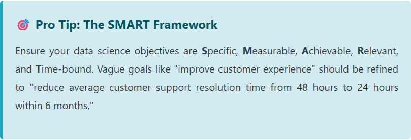
• Problem Framing: Convert vague business needs into specific, solvable data science questions. Is this a classification, regression, clustering, or recommendation problem?
• Success Metrics Definition: Establish clear KPIs that align with business goals, such as reducing customer churn by 15%, improving forecast accuracy by 20%, or increasing conversion rates.
• Feasibility Assessment: Evaluate whether the problem can realistically be solved with available data, resources, and technology.
• Project Scoping: Define timelines, resource requirements, and deliverables.

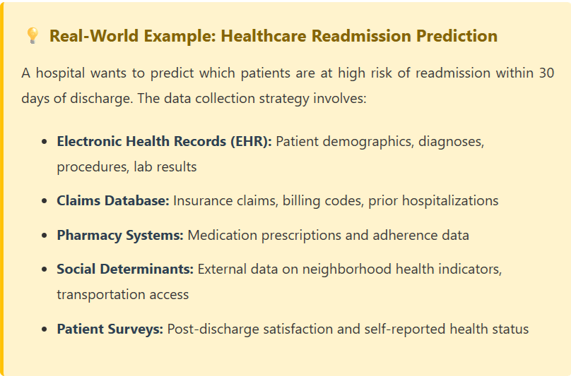
Stage 2: Data Collection and Acquisition

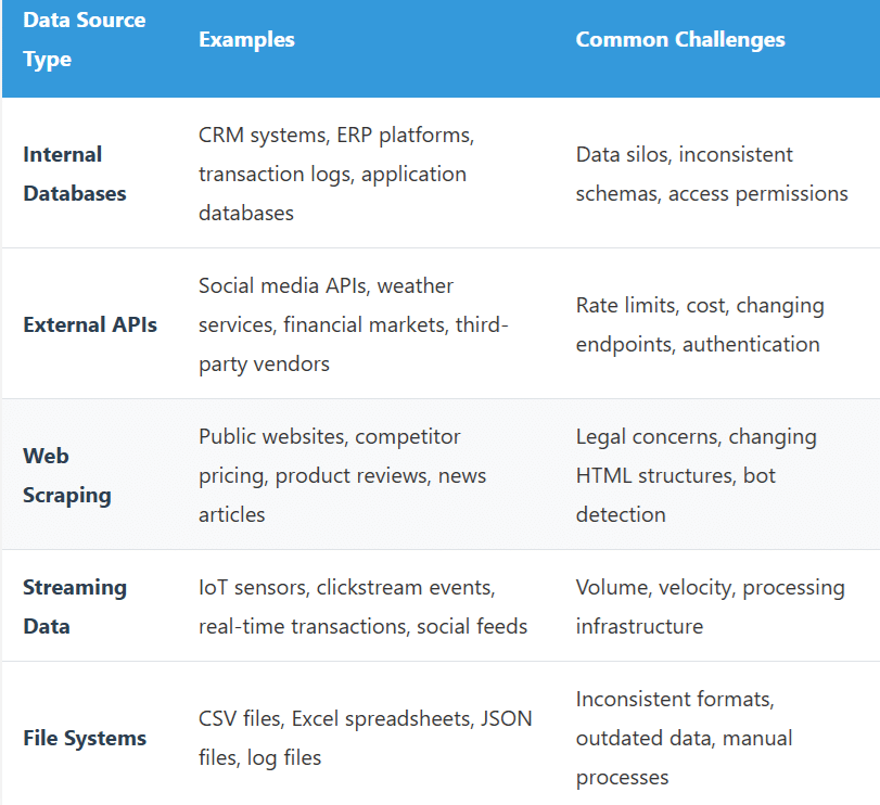
Once you’ve defined the problem, the next critical step is identifying and gathering the data needed to solve it. This stage involves understanding what data exists, where it lives, and how to access it effectively. The quality and relevance of your data will ultimately determine the success of your entire project.

Data Source Categories:

Data Collection Best Practices:

• Data Governance: Ensure compliance with regulations like GDPR, HIPAA, or CCPA when collecting personal information.
• Documentation: Maintain detailed metadata about data sources, collection methods, and update frequencies.
• Automation: Build robust data pipelines using tools like Apache Airflow, Prefect, or cloud-native solutions.
• Version Control: Track different versions of datasets to ensure reproducibility.
• Data Quality Checks: Implement validation rules at the point of collection to catch issues early.

Stage 3: Data Exploration and Analysis (EDA)

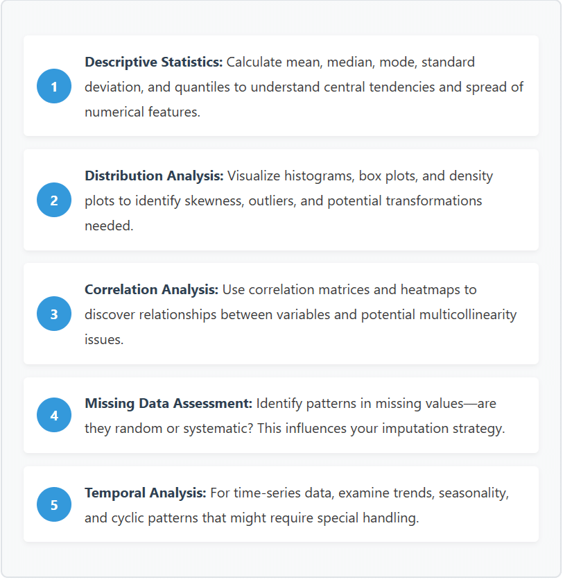
Exploratory Data Analysis (EDA) is where data scientists become detectives, investigating the structure, patterns, and quirks of their datasets. This critical stage helps you understand what you’re working with before jumping into modeling, potentially saving weeks of wasted effort on the wrong approach.

Core EDA Techniques:

# Example Python EDA Code 
import pandas as pd import matplotlib.pyplot as plt 
import seaborn as sns 
# Load and inspect data 
df = pd.read_csv('customer_data.csv') 
print(df.info()) 
print(df.describe()) 
# Check missing values 
missing_summary = df.isnull().sum() 
print(missing_summary[missing_summary > 0]) 
# Visualize distributions 
df.hist(figsize=(15, 10), bins=30) 
plt.tight_layout() plt.show() 
# Correlation heatmap 
plt.figure(figsize=(12, 8)) 
sns.heatmap(df.corr(), annot=True, cmap='coolwarm', center=0) 
plt.title('Feature Correlation Matrix') plt.show()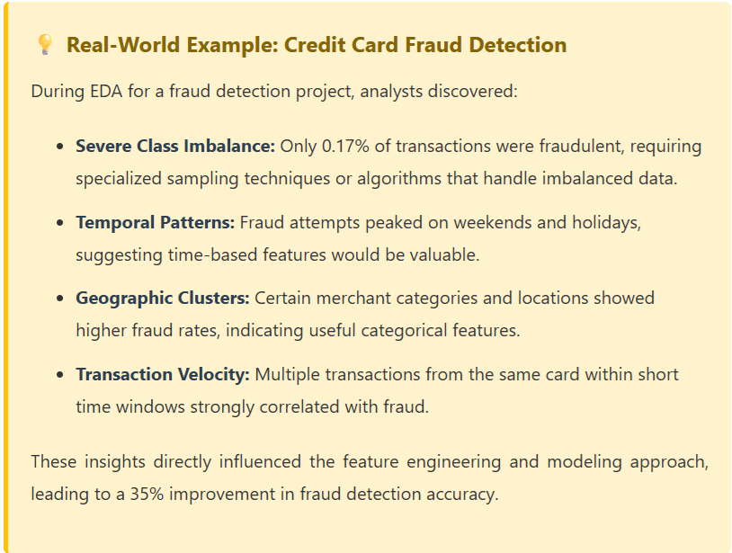

Stage 4: Data Preparation and Feature Engineering

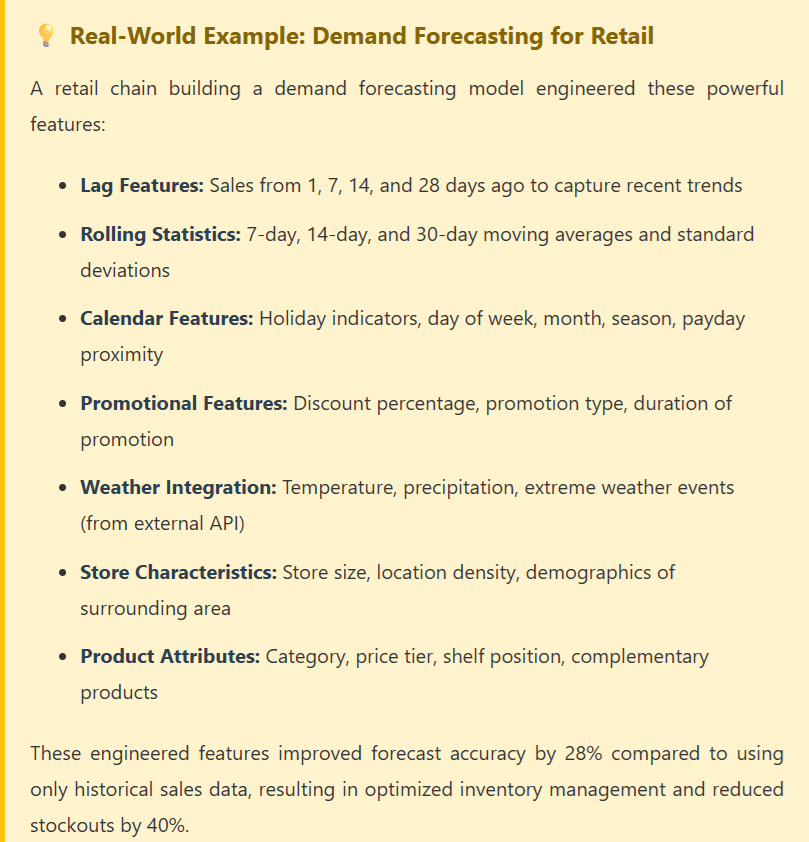
Often consuming 60-80% of a data scientist’s time, data preparation and feature engineering are where raw data is transformed into high-quality inputs that machine learning models can effectively learn from. This stage can make or break your model’s performance—great features with a simple algorithm often outperform poor features with a sophisticated model.

Data Cleaning Operations:

• Handling Missing Values: Implement strategies like mean/median imputation, forward/backward filling for time series, or advanced techniques like KNN imputation or MICE (Multiple Imputation by Chained Equations).
• Outlier Treatment: Decide whether to remove, cap, or transform outliers based on domain knowledge and their impact on model performance.
• Data Type Conversion: Ensure proper data types—dates as datetime objects, categories as categorical, numbers as numeric.
• Duplicate Removal: Identify and handle duplicate records that could bias model training.
• Inconsistency Resolution: Standardize values like “NY”, “New York”, and “new york” to a single representation.

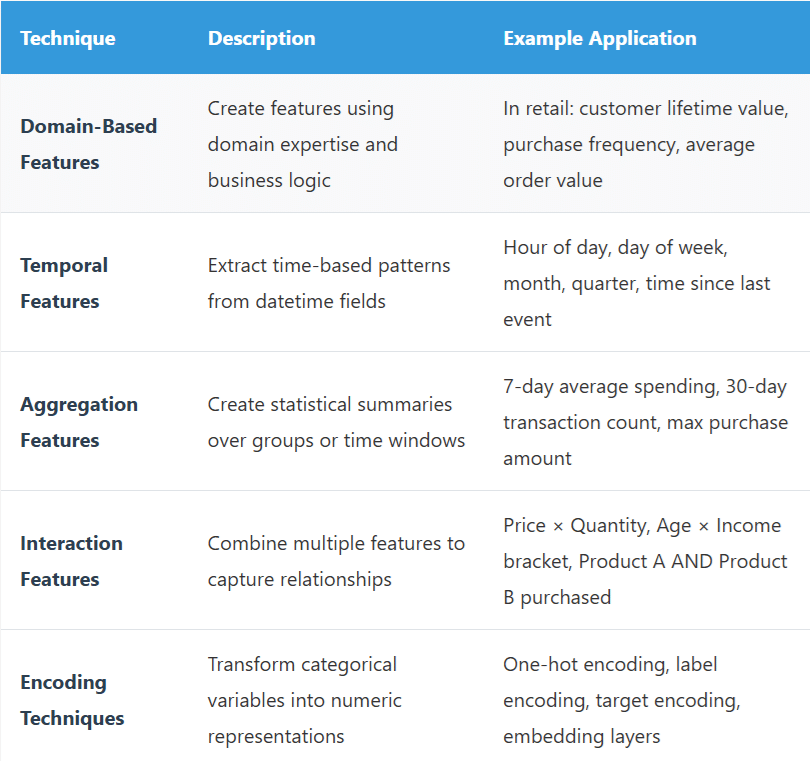
Feature Engineering Techniques:

Stage 5: Model Development and Training

With clean, well-engineered features in hand, it’s time to build and train machine learning models. This stage involves selecting appropriate algorithms, tuning hyperparameters, and iteratively improving model performance through systematic experimentation.

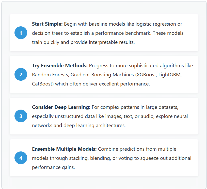
Model Selection Strategy:

Choosing the right algorithm depends on several factors including your problem type, data characteristics, interpretability requirements, and computational constraints. Here’s a strategic approach:

Training Best Practices:

• Train-Validation-Test Split: Properly partition your data (typically 70-20-10 or 60-20-20) to prevent overfitting and get honest performance estimates.
• Cross-Validation: Use k-fold cross-validation to get more robust performance estimates, especially with smaller datasets.
• Hyperparameter Tuning: Systematically search for optimal hyperparameters using grid search, random search, or Bayesian optimization.
• Regularization: Apply techniques like L1/L2 regularization, dropout, or early stopping to prevent overfitting.
• Experiment Tracking: Use MLflow, Weights & Biases, or Neptune.ai to track experiments, compare model versions, and ensure reproducibility.

# Example Model Training Pipeline 
from sklearn.model_selection import train_test_split 
from sklearn.ensemble import RandomForestClassifier 
from xgboost import XGBClassifier import mlflow 
# Split data 
X_train, X_test, y_train, y_test = train_test_split( X, y, test_size=0.2, random_state=42, stratify=y ) 
# Start MLflow experiment 
mlflow.start_run() 
# Train baseline model 
rf_model = RandomForestClassifier(n_estimators=100, random_state=42) 
rf_model.fit(X_train, y_train) 
rf_score = rf_model.score(X_test, y_test) 
mlflow.log_metric("rf_accuracy", rf_score) 
# Train XGBoost model 
xgb_model = XGBClassifier( n_estimators=200, max_depth=6, learning_rate=0.1, random_state=42 ) xgb_model.fit(X_train, y_train) 
xgb_score = xgb_model.score(X_test, y_test) 
mlflow.log_metric("xgb_accuracy", xgb_score) 
# Log best model 
best_model = xgb_model if xgb_score > rf_score else rf_model mlflow.sklearn.log_model(best_model, "best_model") 
mlflow.end_run()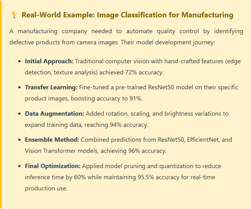

Stage 6: Model Evaluation and Validation

Model evaluation goes far beyond looking at a single accuracy score. This stage involves comprehensively assessing your model’s performance across multiple dimensions, understanding its limitations, and validating that it meets business requirements before deployment.

Key Evaluation Metrics by Problem Type:

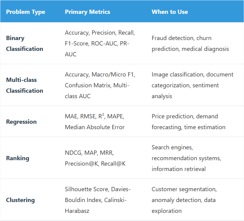
Comprehensive Validation Checklist:

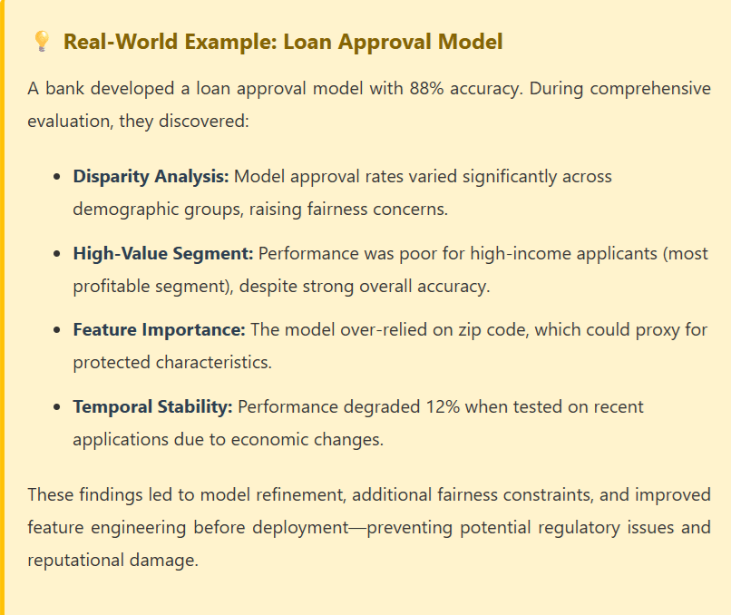
• Business Metric Alignment: Ensure model metrics translate to actual business value. A 95% accurate model is useless if it doesn’t move the needle on revenue, costs, or customer satisfaction.
• Fairness and Bias Testing: Evaluate model performance across different demographic groups to ensure equitable treatment and compliance with regulations.
• Robustness Analysis: Test model behavior with edge cases, adversarial inputs, and data distribution shifts.
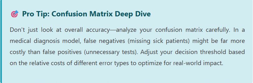
• Error Analysis: Deeply investigate misclassifications or high-error predictions to identify systematic failures and improvement opportunities.
• Computational Efficiency: Measure inference latency and resource consumption to ensure production feasibility.
• Interpretability Assessment: For high-stakes decisions, use SHAP values, LIME, or other explainability techniques to understand model reasoning.

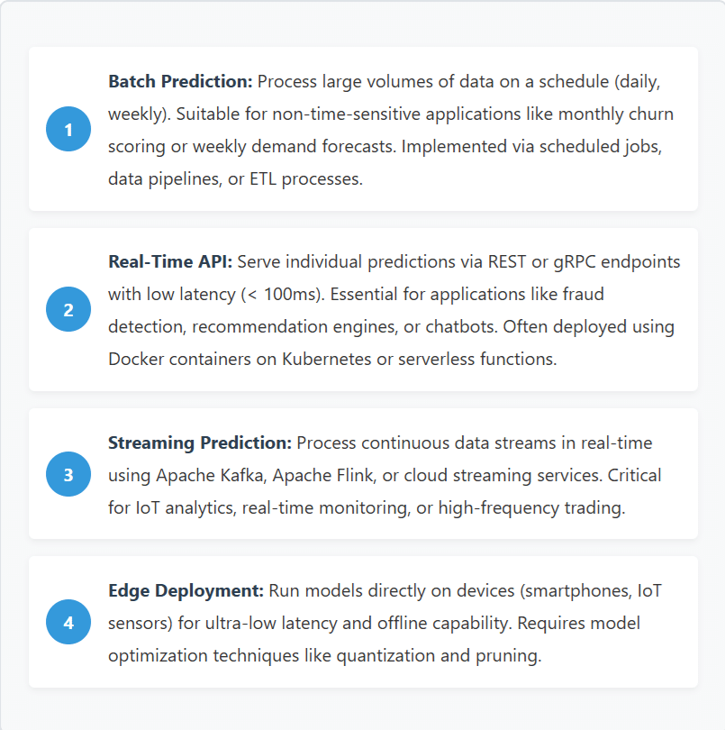
Stage 7: Model Deployment and Production

Deploying machine learning models to production is where data science delivers tangible business value. This stage transforms your experimental notebook code into robust, scalable systems that serve predictions to end-users or business processes reliably and efficiently.

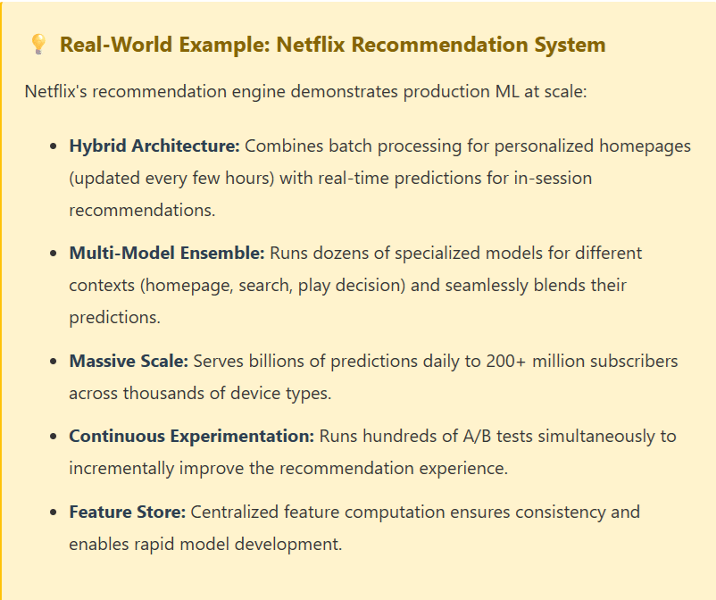
Deployment Architectures:

Production MLOps Best Practices:

• Containerization: Package models with their dependencies in Docker containers for consistent deployment across environments.
• CI/CD Pipelines: Automate testing, validation, and deployment workflows to enable rapid, safe iterations.
• Version Control: Track model versions, training data, and code together to ensure complete reproducibility and easy rollbacks.
• A/B Testing: Gradually roll out new models by serving them to a subset of traffic, comparing against baseline before full deployment.
• Canary Deployments: Deploy new versions incrementally to detect issues before impacting all users.
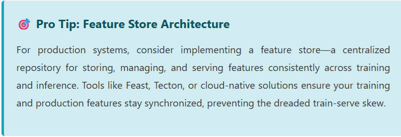
• Feature Serving: Implement consistent feature computation between training and inference to prevent train-serve skew.
• Scalability: Design for horizontal scaling to handle traffic spikes and growing user bases.
• Caching: Cache frequently requested predictions to reduce latency and computational costs.

# Example: Deploy Model as REST API with FastAPI 
from fastapi import FastAPI 
from pydantic import BaseModel 
import joblib 
import numpy as np 
# Load trained model 
model = joblib.load('churn_model.pkl') 
app = FastAPI() 
class PredictionInput(BaseModel): tenure: int monthly_charges: float total_charges: float contract_type: str payment_method: str @app.post("/predict") async def predict_churn(input_data: PredictionInput): 
# Preprocess features features = np.array([[ input_data.tenure, input_data.monthly_charges, input_data.total_charges, encode_contract(input_data.contract_type), encode_payment(input_data.payment_method) ]]) 
# Get prediction probability = model.predict_proba(features)[0][1] prediction = "High Risk" if probability > 0.5 else "Low Risk" return { "churn_probability": float(probability), "risk_category": prediction, "model_version": "v2.3.1" }

Stage 8: Monitoring and Maintenance

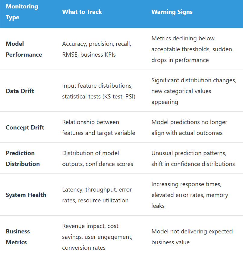
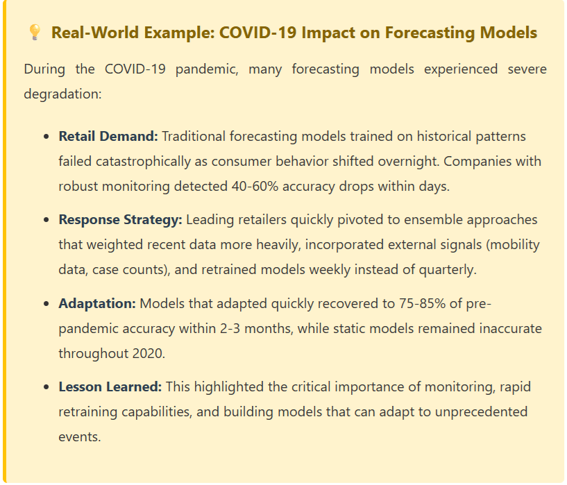
Deployment is not the finish line—it’s the starting line for ongoing model maintenance. Machine learning models degrade over time as data distributions shift, user behavior changes, and business contexts evolve. Continuous monitoring and maintenance ensure your models remain accurate, reliable, and valuable.

Key Monitoring Dimensions:

Maintenance Strategies:

• Automated Retraining: Set up pipelines that automatically retrain models on fresh data when performance degrades or on a regular schedule.
• Online Learning: Implement continuous learning systems that update models incrementally with new data without full retraining.
• Model Registry: Maintain a version-controlled repository of all model artifacts, enabling quick rollbacks if issues arise.
• Alerting Systems: Configure alerts for anomalies in performance, data quality, or system health to enable rapid response.
• Feedback Loops: Collect ground truth labels from production predictions to assess real-world performance and identify areas for improvement.
• Regular Audits: Conduct periodic reviews of model fairness, bias, and alignment with business objectives.

Best Practices and Common Pitfalls

Essential Best Practices:

• Start with the End in Mind: Define deployment requirements and constraints early. Understanding production realities prevents building models that can’t actually be deployed.
• Embrace Iteration: The data science lifecycle is rarely linear. Expect to cycle back through stages as you learn more about your data and problem.
• Document Everything: Maintain comprehensive documentation of decisions, experiments, and findings. Your future self and teammates will thank you.
• Collaborate Cross-Functionally: Work closely with domain experts, engineers, product managers, and business stakeholders throughout the process.
• Prioritize Reproducibility: Use version control for code, data, and models. Set random seeds and document environment configurations.
• Build for Maintainability: Write clean, modular code with proper testing. Complex, clever solutions are hard to maintain and debug in production.
• Balance Complexity and Performance: Sometimes a simple, interpretable model that’s easy to maintain is better than a complex model with marginally better accuracy.

Common Pitfalls to Avoid:

• Data Leakage: Accidentally including information in training data that wouldn’t be available at prediction time, leading to overly optimistic performance estimates.
• Ignoring Class Imbalance: Treating imbalanced classification problems with standard approaches, resulting in models that predict only the majority class.
• Overfitting to Validation Data: Repeatedly tuning hyperparameters based on validation performance, essentially using it as a second training set.
• Focusing Only on Accuracy: Optimizing for a single metric without considering business impact, fairness, or computational constraints.
• Neglecting Feature Engineering: Jumping straight to complex algorithms without investing time in creating meaningful features from domain knowledge.
• Insufficient Testing: Deploying models without comprehensive testing across edge cases, different user segments, and failure scenarios.
• Poor Communication: Presenting results in technical jargon that business stakeholders can’t understand or act upon.
• Underestimating Deployment Complexity: Assuming deployment is trivial, only to discover infrastructure, latency, or integration challenges.

Conclusion: Mastering the Data Science Journey

The data science lifecycle provides a structured roadmap for transforming business problems into production-ready solutions that deliver measurable value. While the eight stages we’ve explored—from problem definition through monitoring and maintenance—offer a logical progression, real-world projects require flexibility, iteration, and continuous learning.

Success in data science isn’t just about building accurate models; it’s about understanding business context, engineering meaningful features, ensuring fairness and reliability, and maintaining systems that continue delivering value over time. The best data scientists are those who can navigate the entire lifecycle, communicating effectively with stakeholders, anticipating production challenges, and building solutions that scale.

As you apply this framework to your own projects, remember that each stage builds upon the previous one. Rushing through early stages like problem definition or data exploration often leads to wasted effort later. Conversely, investing time upfront in understanding your data, engineering thoughtful features, and planning for production pays compound dividends throughout the project lifecycle.

The field of data science continues evolving rapidly, with new tools, techniques, and best practices emerging regularly. However, the fundamental lifecycle principles remain constant: start with clear business objectives, leverage high-quality data, build robust models, deploy with confidence, and monitor continuously. Master these fundamentals, stay curious, and you’ll be well-equipped to tackle the data science challenges of today and tomorrow.