Excel is an indispensable tool for any analyst, and mastering its functions can dramatically boost your productivity and the quality of your insights. Among the most powerful yet straightforward functions is SUMIF. It allows you to sum values in a range that meet a specific criterion, making it a go-to for conditional summing. Whether you’re a seasoned data professional or just starting your analytical journey, a deep understanding of SUMIF is non-negotiable.
This comprehensive guide will walk you through 10 practical SUMIF examples, from basic applications to more advanced techniques. We will explore how to use numbers, text, dates, wildcards, and even combine it with other functions to solve real-world data analysis problems. By the end of this article, you will have the confidence to apply the SUMIF function to nearly any dataset.
To help you follow along and practice, we have included a downloadable Excel file containing all the data and formulas discussed in this post.
What is the SUMIF Function in Excel?
Before we dive into the examples, let’s quickly break down the SUMIF function’s syntax. The function requires three arguments (or inputs) to work correctly:
=SUMIF(range, criteria, [sum_range])
Let’s look at each component:
range(required): This is the range of cells you want to evaluate against your criteria. For example, a column of product names or a list of regions.criteria(required): This is the condition that determines which cells to sum. It can be a number, text, a logical expression, or a cell reference. For instance, the text “East” or the expression “>100”.[sum_range](optional): This is the actual range of cells to sum. If you omit this argument, Excel will sum the cells specified in therangeargument. This is useful when the cells you are evaluating are the same ones you want to sum (e.g., summing all numbers greater than 50 in a column of numbers).
Now, let’s bring this function to life with some real-world Excel tips for data analysis.
Getting Started: The Sample Dataset
For all our examples, we will use the following sales dataset. It contains information about Order ID, Order Date, Region, Product, Units Sold, and Total Revenue. This structure is common in many business analyses, making the examples easily transferable to your own work.
Sample Sales Data
| Order ID | Order Date | Region | Product | Units Sold | Total Revenue |
|---|---|---|---|---|---|
| 101 | 01-Jan-24 | North | Alpha | 50 | $5,000 |
| 102 | 05-Jan-24 | South | Bravo | 30 | $4,500 |
| 103 | 12-Jan-24 | East | Charlie | 25 | $3,125 |
| 104 | 15-Jan-24 | North | Bravo | 40 | $6,000 |
| 105 | 21-Jan-24 | West | Alpha | 60 | $6,000 |
| 106 | 03-Feb-24 | South | Charlie | 20 | $2,500 |
| 107 | 10-Feb-24 | East | Bravo | 35 | $5,250 |
| 108 | 18-Feb-24 | North | Alpha | 55 | $5,500 |
| 109 | 25-Feb-24 | West | Charlie | 15 | $1,875 |
| 110 | 02-Mar-24 | South | Alpha | 65 | $6,500 |
Example 1: Sum Based on a Simple Text Criterion
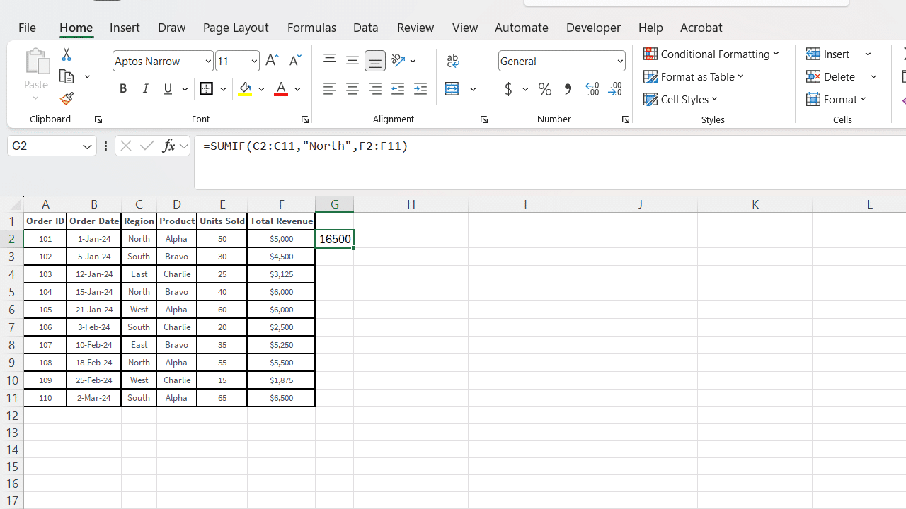
This is the most common use of the SUMIF function. Let’s say we want to calculate the total revenue generated from the “North” region.
Objective: Find the total revenue for the North region.
- Formula:
=SUMIF(C2:C11, "North", F2:F11) range:C2:C11(the Region column)criteria:"North"(the specific text we are looking for)sum_range:F2:F11(the Total Revenue column)
Explanation:
The formula scans cells C2 through C11. For every cell that contains the exact text “North” (rows for Order IDs 101, 104, and 108), it finds the corresponding value in the sum_range (F2:F11) and adds them up.
Calculation:
$5,000 (from row 2) + $6,000 (from row 5) + $5,500 (from row 9) = $16,500
Pro Tip: Instead of hardcoding the criteria like “North” into the formula, you can reference a cell. If you type “North” into cell H2, the formula becomes =SUMIF(C2:C11, H2, F2:F11). This makes your spreadsheet more dynamic and user-friendly.
Example 2: Sum Based on a Numeric Criterion (Greater Than)
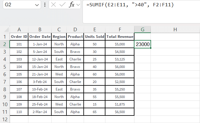
SUMIF is excellent for filtering and summing numbers. Let’s find the total revenue from all orders where more than 40 units were sold.
Objective: Sum the revenue for orders with more than 40 units sold.
- Formula:
=SUMIF(E2:E11, ">40", F2:F11) range:E2:E11(the Units Sold column)criteria:">40"(the logical expression for “greater than 40”)sum_range:F2:F11(the Total Revenue column)
Explanation:
This formula evaluates the “Units Sold” column. It sums the revenue for orders 101 (50 units), 105 (60 units), 108 (55 units), and 110 (65 units). Note that the logical operator (>) and the number (40) must be enclosed in double quotes.
Calculation:
$5,000 + $6,000 + $5,500 + $6,500 = $23,000
Example 3: Sum Based on a “Not Equal To” Criterion
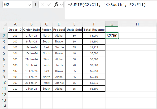
Sometimes, you need to sum everything except for values that meet a certain condition. The “not equal to” operator, <>, is perfect for this. Let’s calculate the total revenue from all regions except “South”.
Objective: Sum all revenue not generated by the South region.
- Formula:
=SUMIF(C2:C11, "<>South", F2:F11) range:C2:C11(the Region column)criteria:"<>South"(the “not equal to” condition)sum_range:F2:F11(the Total Revenue column)
Explanation:
The formula looks through the Region column and adds up the revenue for any row where the region is not “South”. This is a key part of any Excel SUMIF tutorial: learning how to exclude data.
Calculation:
This will sum the revenue for all orders except 102, 106, and 110. The total revenue is $46,250. The revenue from South is $4,500 + $2,500 + $6,500 = $13,500. So, $46,250 – $13,500 = $32,750.
Example 4: Using Wildcards for Partial Text Matches
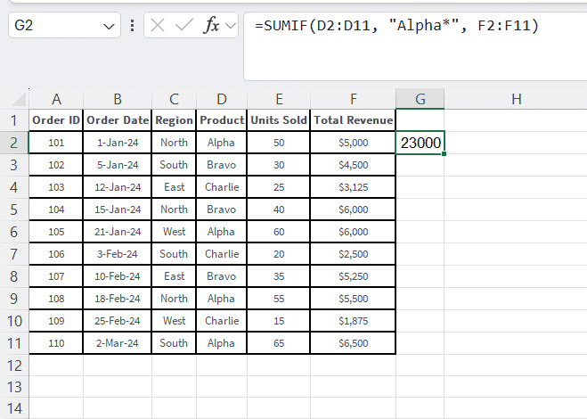
What if you need to sum values based on a partial text match? This is where wildcards come in. The asterisk (*) represents any number of characters, while the question mark (?) represents a single character.
Let’s say our product names were more complex, like “Alpha-Widget” and “Alpha-Gadget”. We want to sum the revenue for all products that start with “Alpha”.
Objective: Sum revenue for all products starting with “Alpha”. (Using our sample data, this will just be “Alpha”).
- Formula:
=SUMIF(D2:D11, "Alpha*", F2:F11) range:D2:D11(the Product column)criteria:"Alpha*"(matches any text starting with “Alpha”)sum_range:F2:F11(the Total Revenue column)
Explanation:
The asterisk acts as a wildcard. The criteria "Alpha*" tells Excel to find any cell in the range that begins with the text “Alpha”, regardless of what follows. This is incredibly useful for categorizing data that isn’t perfectly clean.
Calculation:
The formula finds “Alpha” in rows for orders 101, 105, 108, and 110.
$5,000 + $6,000 + $5,500 + $6,500 = $23,000
Imagine you wanted to sum revenue for all products ending in “vo”. You would use the criteria "*vo". For our data, this would match “Bravo”.
Example 5: Summing Based on a Date Criterion
Working with dates is a common task for analysts. SUMIF can handle date criteria just as easily as text or numbers. Let’s calculate the total revenue for all orders placed after January 31, 2024.
Objective: Sum revenue for orders placed in February 2024 or later.
- Formula:
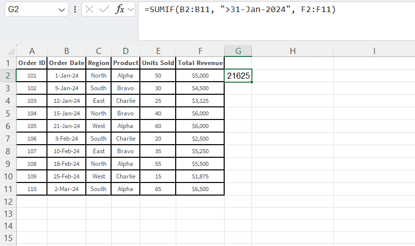
=SUMIF(B2:B11, ">31-Jan-2024", F2:F11) range:B2:B11(the Order Date column)criteria:">31-Jan-2024"(the date condition)sum_range:F2:F11(the Total Revenue column)
Explanation:
Similar to numeric criteria, date criteria must be enclosed in quotes. Excel is smart enough to interpret “31-Jan-2024” as a date. This formula will sum the revenue for all orders with a date in February and March.
Calculation:
This sums the revenue for orders 106, 107, 108, 109, and 110.
$2,500 + $5,250 + $5,500 + $1,875 + $6,500 = $21,625
Pro Tip: You can also use the TODAY() function to create dynamic date-based summaries. For example, to sum revenue from the last 30 days, your criteria might look like ">"&TODAY()-30.
Example 6: Summing Blank or Non-Blank Cells
Data is rarely perfect. You will often encounter datasets with missing information. The SUMIF function for analysts is invaluable for handling these gaps.
Objective A: Sum the revenue for orders where the region is not specified (is blank).
Let’s pretend the region for order 103 is blank.
- Formula:
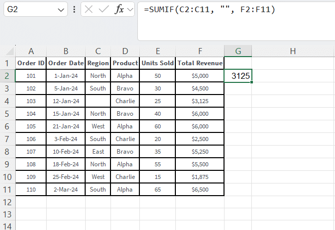
=SUMIF(C2:C11, "", F2:F11) criteria:""(two double quotes with nothing in between represents a blank cell)
Explanation:
This formula identifies any blank cells in the region column and sums the corresponding revenue. In our modified scenario, this would return $3,125.
Objective B: Sum the revenue for orders where the region is specified (is not blank).
- Formula:
=SUMIF(C2:C11, "<>", F2:F11) criteria:"<>"(the “not equal to” operator used alone represents non-blank cells)
Explanation:
This formula does the opposite. It sums the revenue for any row that has a value in the region column. In our modified scenario, this would sum the revenue for all orders except 103, for a total of $48,125.
Example 7: Omitting the [sum_range] Argument
As mentioned in the syntax breakdown, the sum_range is optional. If you omit it, SUMIF will sum the values in the range argument. This is useful when the condition and the sum values are in the same column.
Objective: Sum all revenue amounts that are greater than $5,000.
- Formula:
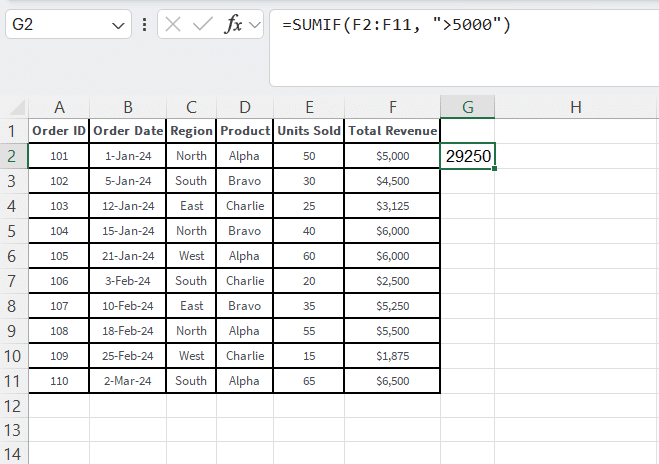
=SUMIF(F2:F11, ">5000") range:F2:F11(the Total Revenue column)criteria:">5000"(the condition to check)sum_range: Omitted. Excel will sum the cells in therange(F2:F11) that meet the criteria.
Explanation:
The formula looks at each cell in F2:F11. If a cell’s value is greater than 5000, it is included in the sum.
Calculation:
$6,000 + $6,000 + $5,250 + $5,500 + $6,500 = $29,250
Example 8: Using a Cell Reference in the Criteria
Hardcoding criteria into formulas is generally bad practice. It makes them difficult to update. A more flexible approach is to reference a cell that contains the criterion.
Let’s revisit our first example. We want to sum revenue by region, but we want to create a small summary table where a user can type the region name.
Setup:
- In cell H2, type the header “Region”.
- In cell I2, type the header “Total Revenue”.
- In cell H3, you will type the region you want to summarize (e.g., “East”).
Objective: Sum revenue based on the region typed into cell H3.
- Formula (in cell I3):
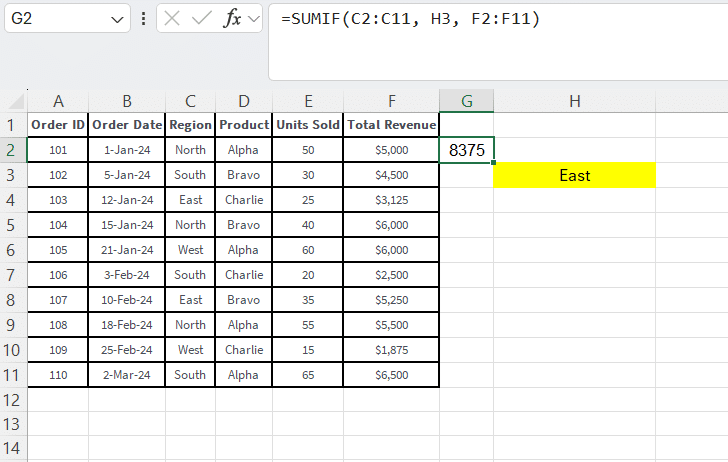
=SUMIF(C2:C11, H3, F2:F11) range:C2:C11(Region column)criteria:H3(a reference to the cell containing our criterion)sum_range:F2:F11(Total Revenue column)
Explanation:
Now, the formula in I3 will dynamically update based on the value in H3. If you type “East” in H3, it will calculate the sum for the East region ($3,125 + $5,250 = $8,375). If you change H3 to “West”, the formula will automatically recalculate to show the sum for the West region ($6,000 + $1,875 = $7,875). This is a fundamental concept for building interactive dashboards in Excel.
Example 9: Combining an Operator with a Cell Reference
You can take the previous example a step further by combining a logical operator (like >, <, or <>) with a cell reference. This requires a slightly different syntax using the ampersand (&) to concatenate the operator and the cell reference.
Setup:
- In cell H5, type a revenue threshold, for example,
5000.
Objective: Sum all revenue amounts greater than the value entered in cell H5.
- Formula:
=SUMIF(F2:F11, ">"&H5) range:F2:F11criteria:">"&H5(concatenates the “>” operator with the value in H5)sum_range: Omitted.
Explanation:
The ampersand joins the string ">" with the value from cell H5. If H5 contains 5000, Excel interprets the criteria as ">5000". If you change the value in H5 to 6000, the formula will automatically update to sum only revenues greater than $6,000, without you ever having to edit the formula itself. This is an essential technique for advanced Excel tips for data analysis.
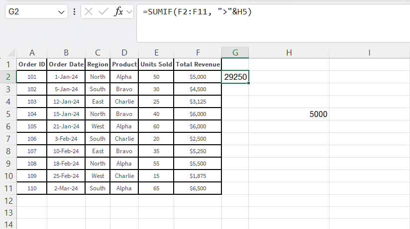
Calculation (with H5 = 5000):
$6,000 + $6,000 + $5,250 + $5,500 + $6,500 = $29,250
Example 10: The Limitation of SUMIF and the Introduction to SUMIFS
The SUMIF function is powerful, but it has one major limitation: it can only handle a single criterion. What if you need to sum the revenue for “Product Alpha” sold specifically in the “North” region? You have two conditions.
This is where the SUMIFS function comes in. The syntax is slightly different and more flexible:
=SUMIFS(sum_range, criteria_range1, criteria1, [criteria_range2, criteria2], ...)
Notice that the sum_range comes first in SUMIFS.
Objective: Sum the revenue for “Product Alpha” in the “North” region.
- Formula:
=SUMIFS(F2:F11, C2:C11, "North", D2:D11, "Alpha") sum_range:F2:F11(the range to sum)criteria_range1:C2:C11(the Region column)criteria1:"North"criteria_range2:D2:D11(the Product column)criteria2:"Alpha"
Explanation:
SUMIFS checks both conditions for each row. A row’s revenue is only added to the total if the Region is “North” and the Product is “Alpha”. This is the natural progression from SUMIF and a vital function for analysts who need to perform more complex filtering.
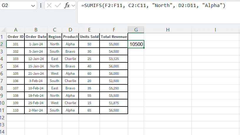
Calculation:
The formula identifies rows for orders 101 and 108 as meeting both criteria.
$5,000 + $5,500 = $10,500
Understanding this limitation and knowing when to switch to SUMIFS is the mark of a proficient Excel user. While this article focuses on SUMIF, recognizing its boundaries is a crucial takeaway. You can download the working file from below.
Frequently Asked Questions (FAQs) about SUMIF
Q1: What is the difference between SUM, SUMIF, and SUMIFS?
- SUM: Adds all numbers in a range of cells.
=SUM(A1:A10) - SUMIF: Sums the cells in a range that meet a single specified condition.
=SUMIF(A1:A10, ">50", B1:B10) - SUMIFS: Sums the cells in a range that meet multiple specified conditions.
=SUMIFS(C1:C10, A1:A10, "North", B1:B10, ">50")
Q2: Is the SUMIF function case-sensitive?
No, the SUMIF function is not case-sensitive. The criteria "North", "north", and "NORTH" will all produce the same result. This is generally helpful, but if you need case-sensitive summing, you would need to use a more complex formula involving the SUMPRODUCT and EXACT functions.
Q3: Can SUMIF be used across different worksheets?
Yes. You can reference ranges on other sheets within the same workbook. The syntax would look like this: =SUMIF(Sheet2!A1:A10, "Criteria", Sheet2!B1:B10). Just be sure to include the sheet name followed by an exclamation mark before the range reference.
Q4: Why is my SUMIF formula returning 0?
A zero result usually means one of three things:
- No cells in your
rangemeet thecriteria. Double-check for typos or extra spaces in your criteria. - The
sum_rangecontains text or blank cells for the rows that meet the criteria. - The numbers in your
sum_rangeare formatted as text. You can fix this by selecting the column, going to the Data tab, and using the “Text to Columns” feature.
Q5: How do I use SUMIF with dates?
As shown in Example 5, you enclose the date and any logical operator in double quotes (e.g., ">01-Jan-2024"). For more flexibility, it’s often better to reference a cell containing the date, like ">"&H1, where H1 holds the date value. This prevents issues with regional date formatting.
Test Your SUMIF Knowledge: Quiz
Ready to see what you’ve learned? Use the sample dataset provided at the beginning of the article to answer these questions.
SUMIF Knowledge Quiz
Quiz Answers: 1-B, 2-B, 3-C, 4-C, 5-B, 6-B, 7-C
Conclusion and Next Steps
The SUMIF function is a cornerstone of effective data analysis in Excel. By mastering these 10 examples, you have built a solid foundation for performing conditional sums on text, numbers, dates, and even messy data with blanks or partial matches. You have also learned how to make your spreadsheets more dynamic by using cell references in your criteria and, crucially, when to graduate from SUMIF to the more powerful SUMIFS for handling multiple conditions.
The best way to solidify your understanding is through practice. Be sure to download the companion Excel file that includes all the datasets and formulas from this article. Try to replicate the results and then adapt the formulas to answer new questions about the data. For example, can you calculate the total units sold for “Product Bravo”? Or the total revenue for orders under $5,000?
As you grow more comfortable, you will find that SUMIF becomes an automatic part of your analytical toolkit, saving you time and enabling you to uncover valuable insights from your data with speed and precision.